<?xml version="1.0" encoding="utf-8"?><feed xmlns="http://www.w3.org/2005/Atom" ><generator uri="https://jekyllrb.com/" version="3.10.0">Jekyll</generator><link href="/feed.xml" rel="self" type="application/atom+xml" /><link href="/" rel="alternate" type="text/html" /><updated>2026-08-20T05:17:49+00:00</updated><id>/feed.xml</id><title type="html">Huihang Liu</title><subtitle></subtitle><entry><title type="html">Summary on Causal Inference for Time Series Analysis</title><link href="/policycausal/" rel="alternate" type="text/html" title="Summary on Causal Inference for Time Series Analysis" /><published>2022-08-21T00:00:00+00:00</published><updated>2022-08-21T00:00:00+00:00</updated><id>/policycausal</id><content type="html" xml:base="/policycausal/"><![CDATA[<h1 id="时间序列中的因果推断">时间序列中的因果推断</h1>

<h2 id="我们想要了解的问题">我们想要了解的问题</h2>

<ul>
  <li>问题背景与数据的描述
    <ul>
      <li>数据维度, 数据类型, 范围</li>
      <li>数据的实际意义</li>
      <li>变量之间直观上存在的关系</li>
    </ul>
  </li>
  <li>目标的描述
    <ul>
      <li>是否进行效果评估 (或政策评估, 或处理效应估计)?</li>
      <li>是否需要进行假设检验?</li>
      <li>是否需要根据估计效果, 构建最优策略?</li>
    </ul>
  </li>
  <li>预想的结果</li>
  <li>建议
    <ul>
      <li>能否进行随机化的效果评估, 进行 A/B test? 因为随机化实验可以极大简化因果推断.</li>
    </ul>
  </li>
</ul>

<p><a href="https://huihangliu.github.io/policycausal/">这是本文的 HTML 版本</a>, 更方便阅读. 下面是一些方法的总结.</p>

<h2 id="summary-on-causal-inference-for-time-series-analysis">Summary on Causal Inference for Time Series Analysis</h2>

<p>In this note, we summarize the content of the <a href="https://arxiv.org/pdf/2102.05829.pdf"><em>Raha Moraffah et al. (2021)</em></a>. This includes three main types of causal treatment effects estimation for time series data. Currently, we focus on the time-invariant treatment effect and traditional statistics methods.</p>

<p>The state-of-the-art causal treatment effect estimation approaches for time series data can be categorized into three main types:</p>
<ul>
  <li><a href="#1-time-invariant-treatment-effect">1. time-invariant treatment effect</a>;</li>
  <li><a href="#2-time-varying-treatment-effect">2. time-varying treatment effect</a>;</li>
  <li><a href="#3-dynamic-treatment-regimes">3. dynamic treatment regimes</a>.</li>
</ul>

<p>The following figure is a road-map of this note. 
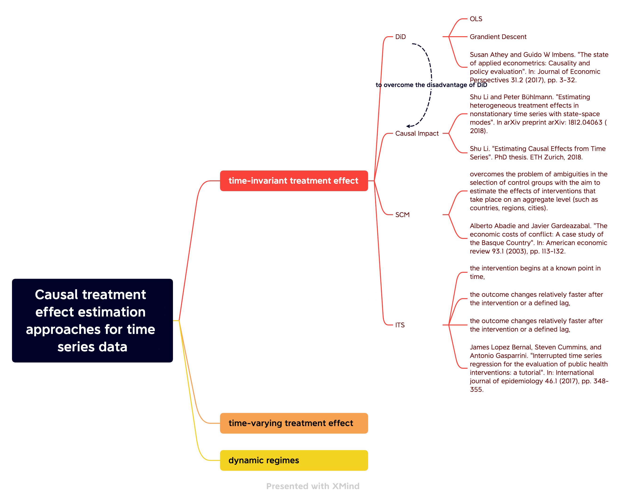
<img src="../assets/Causal.jpg" alt="" /></p>

<h3 id="1-time-invariant-treatment-effect">1 Time-invariant Treatment Effect</h3>
<ul>
  <li><strong><font color="red">What is time-invariant treatment effect?</font></strong>
    <ul>
      <li>A treatment is time-invariant or fixed when it occurs at one specfic point of time and then does not change afterward.</li>
    </ul>
  </li>
  <li>Let $X(t)$ be the time sereis outcome recorded at times $t = 1,2,\dots,n$, and let $A$ be a dichotomous treatment that can take values $a=0$ (untreated) or $a=1$ (treated). We will have:
    <ul>
      <li>$X_a$: the potential outcome for the treatment group (when $a=1$) or control group (when a=0).</li>
      <li>$T$: $1\leq T\leq n$, the time when the intervention occurs.</li>
      <li>$X_{a=1}^c(t&gt;T)$: potential outcome of the treatment group at $t&gt;T$ had it not received the treatment which is known as the <strong>counterfactual outcome</strong>.</li>
    </ul>
  </li>
  <li>In the following section, we will introduce common time-invariant causal effect estimation methods.</li>
</ul>

<h4 id="11-difference-in-difference-did">1.1 Difference in Difference (DID)</h4>

<ul>
  <li>DID is an important tool mostly used by the econometricians to capture the <strong>average causal effect</strong> of the time series data before and after the treatment.</li>
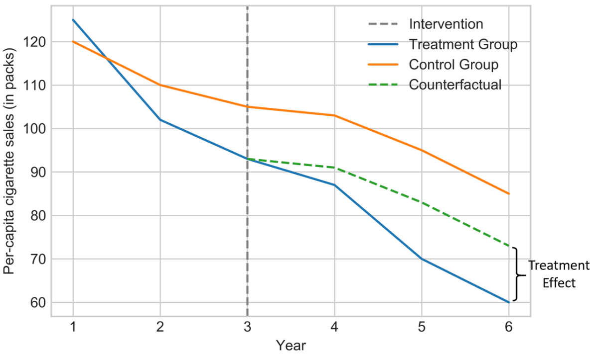
  <li>This tool goes by an <strong>assumption</strong> called <em>common trends</em> or <em>parallel trends</em> that uses the change of the outcome of the control group as a counterfactual for the treatment group in the absence of the treatment.</li>
</ul>

<p>The following figure is an illustration of the DID method. 
<img src="../assets/20220825223025.png" alt="" /></p>

<ul>
  <li>If $t&lt;T$ and $t&gt;T$ denotes the pre- and post- treatment periods, respectively, then we can calculate the DID measure using the average treatment effect of the treated (ATT) metrics as follows<sup id="fnref:1" role="doc-noteref"><a href="#fn:1" class="footnote" rel="footnote">1</a></sup>:</li>
</ul>

\[\begin{aligned}\text{DID}&amp;=\{E[X(t&gt;T)\mid A=1]-E[X(t&lt;T)\mid A=1]\}\\&amp;-\{E[X(t&gt;T)\mid A=0]-E[X(t&lt;T)\mid A=0]\}.\end{aligned}\]

<ul>
  <li>A common solution to model the DID causal effect is to specify a linear regression model for the observed outcome. In case of one intervention and one treatment group we will have:
\(X=\alpha+\beta g+\gamma t +\delta(g\times t)+e,\)</li>
  <li></li>
  <li>$\alpha,\beta,\gamma$ and $\delta$ are the regression coefficients.</li>
  <li>$g$ is a dummy variable indicating the treatment group (1 for treatment and 0 for the control group),</li>
  <li>$t$ is a dummy variable defining the pre- or post-treatment periods (0 for before and 1 for after the treatment time)</li>
  <li>$g\times t$ is the interaction term to count the DID causal effect with $\delta$ being its coefficient</li>
  <li>$e$ is the error term which is independent of other variables.</li>
  <li>The parameters of this regression can be estimated by the available methods solving regression models such as <strong>OLS</strong>.</li>
  <li><strong><font color="red">The disadvantage of DID</font></strong>:
    <ul>
      <li>If it fits to <strong>highly autocorrelated data</strong>, the model <strong>underestimates</strong> the effect of the intervention.</li>
    </ul>
  </li>
  <li>
    <p>For a comprehensive survey on this metric, the author refer the readers to two sutdies provided by Lencher (2011)<sup id="fnref:2" role="doc-noteref"><a href="#fn:2" class="footnote" rel="footnote">2</a></sup> and Bertrand et al. (2004) <sup id="fnref:3" role="doc-noteref"><a href="#fn:3" class="footnote" rel="footnote">3</a></sup>.</p>
  </li>
  <li><strong><font color="red">Related Papers</font></strong>:
    <ul>
      <li>Susan Athey and Guido W Imbens. “<em>The state of applied econometrics: Causality and policy evaluation</em>”. In: <em>Journal of Economic Perspectives 31.2 (2017), pp. 3-32</em>.</li>
      <li>Susan Athey and Guido W Imbens: “<em>Identification and inference in nonlinear difference-in-differences models</em>”. In: <em>Ecnonmetrica 74.2 (2006), pp. 431-497</em>.</li>
      <li>Marianne Bertrand, Esther Duflo, and Sendhil Mullaninathan. “<em>How much should we trust differences-in-differences estimator?</em>” In: <em>The Quarterly journal of economics</em> 119.1 (2004), pp. 249-275.</li>
      <li>Michael Lechner et al. <em>The estimation of causal effects by difference-in-difference methods</em>. Now, 2011.</li>
    </ul>
  </li>
</ul>

<h4 id="12-causal-impact">1.2 Causal Impact</h4>

<ul>
  <li>This method <u>generalizes the concept of the DID</u> and structural time-series model to infer the causal impact of a <strong>discrete intervention</strong> (e.g. the release of a new product). Causal Impact 基于贝叶斯结构时间序列模型, 综合多种信息输入结合自身的时间序列来构造一个策略未上线的虚拟值.</li>
  <li><strong>Advantages</strong>: The assumption of DID on the common trend is weakened. (但依然需要选择合适的控制组.)</li>
  <li><strong>Applications</strong>: It is widely used for various applications such as the impact of vaccines, the environmental impact of aircraft emissions and aviation ful tax, and the impact of mobile phone use on brain cancer.</li>
</ul>

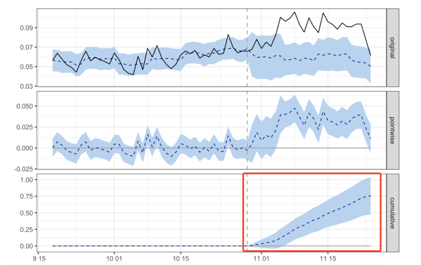
<p>The following figure is an illustration of causal impact method. See <a href="https://maimai.cn/article/detail?fid=1607599585&amp;efid=hQNw4-sFnNlf-k8RrhcNmw">this blog</a> for details.</p>
<ul>
  <li>Subfig 1 (original): 黑色实线为被处理样本的实际观测结果, 蓝色虚线为根据某个控制样本模拟的被处理样本的结果, 蓝色区域为置信区间.</li>
  <li>Subfig 2 (pointwise): 蓝色虚线为被处理样本的实际观测结果与模拟结果的差值, 可以看到实施处理后, 结果的差值是显著为正的.</li>
  <li>
    <p>Subfig 3 (cumulative): 蓝色虚线为实施处理后的累加值, 是持续增大的, 可见处理有明显的正向作用.
<img src="../assets/202208260003001.png" alt="" /></p>
  </li>
  <li>Causal impact learns the relationship between the treatment and control group before any intervention and predicts the counterafctual series after the treatment. This method relies on state-space models as follows:</li>
</ul>

\[\begin{align*}
  \begin{aligned}
    X(t) &amp;= \mu(t)+\beta Z(t)+\upsilon(t)\\\mu(t)&amp;=\mu(t-1)+\delta(t-1)+\omega(t)\\
    \delta(t) &amp;= \delta(t-1)+u(t),
  \end{aligned}
\end{align*}\]

<ul>
  <li>
    <ul>
      <li>$Z(t)$ is the control time series and is related to the treatment time series (i.e. $X(t)$) through the $\beta$ components.</li>
      <li>$\upsilon(t)$, $\omega(t)$ and $u(t)$ are zero-mean noise variables.</li>
      <li>$\mu(t)$ models the temporal correlation in $X(t)$.</li>
      <li>$\delta(t)$ component can be thought of as the slope at time $t-1$ or the expected increase in $\mu$ between times $t-1$ and $t$.</li>
    </ul>
  </li>
  <li>The model is fitted to the observed data $t=1,2,\dots,T$, treating the counterfactual $t=T+1,T+2,\dots,n$ as unobserved random variables.</li>
  <li>The model will compute the posterior distribution of the counterfactual time series. <u>The causal effect is estimated by subtracting the predicted from the observed treated time series.</u></li>
  <li><strong><font color="red">Related Papers</font></strong>:
    <ul>
      <li>Shu Li and Peter Bühlmann. “<em><a href="https://arxiv.org/abs/1812.04063">Estimating heterogeneous treatment effects in nonstationary time series with state-space modes</a></em>”. In <em>arXiv preprint arXiv: 1812.04063 (2020)</em>.</li>
      <li>Shu Li. “<em><a href="https://www.research-collection.ethz.ch/bitstream/handle/20.500.11850/320119/thesis.pdf?sequence=1&amp;isAllowed=y">Estimating Causal Effects from Time Series</a></em>”. PhD thesis. ETH Zurich, 2018.</li>
      <li>Kay H Brodersen et al. “<em>Inferring causal impact using Bayesian structural time-series models</em>”. In: <em>The Annals of Applied Statistics</em> 9.1 (2015), pp. 247-274.</li>
    </ul>
  </li>
</ul>

<h4 id="13-synthetic-control-method-scm">1.3 Synthetic Control Method (SCM)</h4>

<ul>
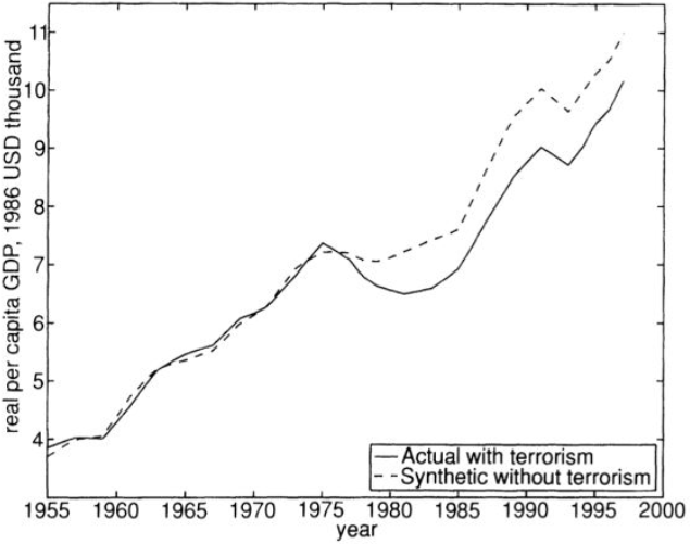
  <li><em>Synthetic Control Method</em> (SCM) introduced by Abadie and Gareazabal in 2003 overcomes the problem of ambiguities in the selection of control groups with the aim to estimate the effects of interventions that take place on an aggregate level (such as countries, regions, cities).</li>
  <li><strong>Advantages</strong>: 完全去除了对控制组的同趋势假设.</li>
  <li>This method has been introduced in the seminar.</li>
  <li><strong><font color="red">Related Papers</font></strong>:
    <ul>
      <li>Alberto Abadie and Javier Gardeazabal. “<em>The economic costs of conflict: A case study of the Basque Country</em>”. In: <em>American economic review 93.1 (2003), pp. 113-132</em>.</li>
    </ul>
  </li>
</ul>

<p>The following figure is an illustration of SCM. See <a href="https://www.zhihu.com/question/43497862/answer/1874867221">this Q&amp;A</a> for details. 
<img src="../assets/20220826001402.png" alt="" /></p>

<h4 id="14-interrupted-time-series-its">1.4 Interrupted Time Series (ITS)</h4>

<p>这里, 我们考虑一项政策或处理, 在全体样本上展开; 即不存在对照组的情况. 
此时, 我们只能分别从处理前后的两段数据中分别拟合模型, 寻找规律. 因此, 这种方法十分依赖于模型设置.</p>

<ul>
  <li><strong>Requirement</strong>:
    <ul>
      <li>the intervention begins at a known point in time,</li>
      <li>the outcome changes relatively faster after the intervention or a defined lag,</li>
      <li>the outcome lasts long enough to measure.</li>
    </ul>
  </li>
  <li>
    <p>The standard ITS model is capable of finding the causal effect of an intervention for only one time series (i.e. when the control unit data is not available). It is built upon a simple idea that the data generating process would have continued in a similar way in the absence of the intervention, which is a special case of <em>regression Discontinuity Design</em> (RDD) when the discontinuity happens in time.</p>
  </li>
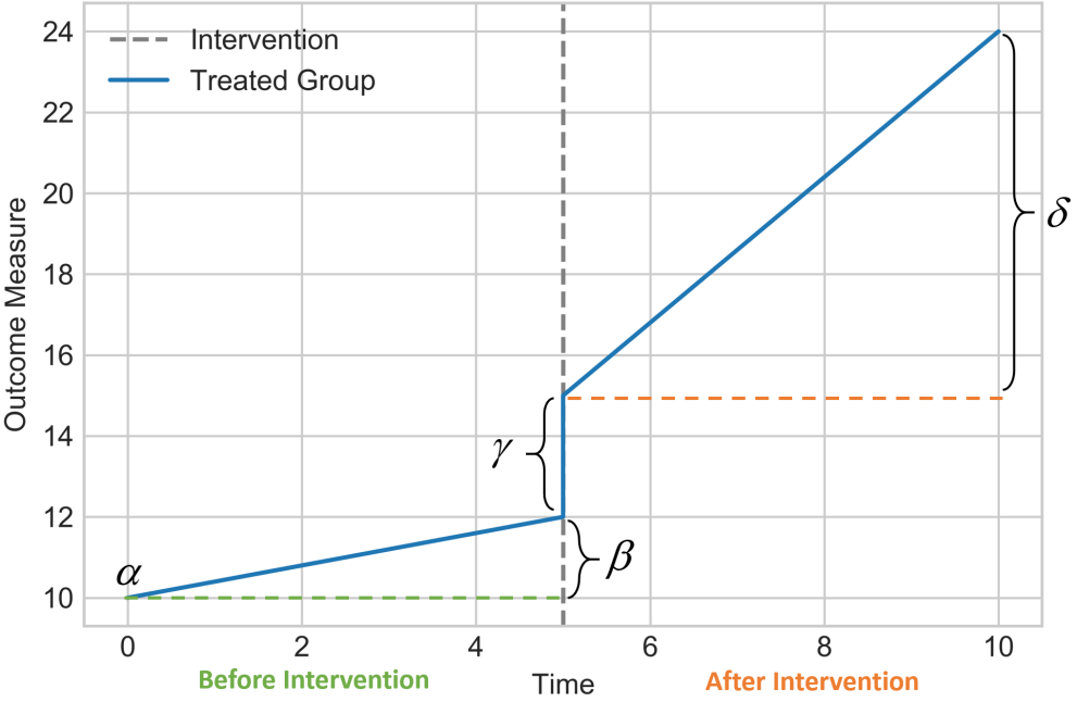
  <li>Therefore, to find immediate changes in the outcome value and the change in the trend of the time series in the post-intervention period compared to the pre-intervention period, “Segmented Regression” (分段回归) is used<sup id="fnref:4" role="doc-noteref"><a href="#fn:4" class="footnote" rel="footnote">4</a></sup>:</li>
</ul>

\[\begin{align*}
  \begin{aligned}
    Y=\alpha+\beta T+\gamma t+\delta (T\times t)+e,
  \end{aligned}
\end{align*}\]

<ul>
  <li>
    <ul>
      <li>$\alpha$ indicates the baseline level at $T=0$,</li>
      <li>$\beta$ represents the baseline trend (i.e. pre-intervention trend),</li>
      <li>$\gamma$ is the immediate level change following the intervention,</li>
      <li>$\delta$ indicates the post-intervention trend</li>
      <li>$e$ is the error.</li>
    </ul>
  </li>
</ul>

<p>The following figure is an illustration of the Standard ITS method.
<img src="../assets/20220825223546.png" alt="" /></p>

<p>See <a href="https://zhuanlan.zhihu.com/p/539045445">this Q&amp;A</a> for details.</p>

<ul>
  <li><strong><font color="red">Related Papers</font></strong>:
    <ul>
      <li>James Lopez Bernal, Steven Cummins, and Antonio Gasparrini. “<em>Interrupted time series regression for the evaluation of public health interventions: a tutorial</em>”. In: <em>International journal of epidemiology 46.1 (2017), pp. 348-355</em>.</li>
      <li>Robert B Penfold and Fang Zhang. “<em>Use of interrupted time series analysis in evaluating health care quality improvements</em>”. In <em>Academic pediatrics 13.6 (2013), S38-S44</em>.</li>
    </ul>
  </li>
</ul>

<h3 id="2-time-varying-treatment-effect">2 Time-varying Treatment Effect</h3>

<ul>
  <li>In this case, A, the treatment variable, would be time-dependent and is recorded throughout all the time, i.e.,</li>
</ul>

\[(A(t)=\{A(1),A(2),\dots,A(n)\}).\]

<h3 id="3-dynamic-treatment-regimes">3 Dynamic Treatment Regimes</h3>
<ul>
  <li>A dynamic treatment regime is a function which takes in treatment and covariate history as arguments and outputs an action to be taken, providing a list of decision rules for how treatment should be allocated over time.</li>
</ul>

<h3 id="4-other-supplementary-machine-learning-method">4 Other Supplementary Machine Learning Method</h3>

<ul>
  <li><em>Double Machine Learning</em> (DML)
    <ul>
      <li>Paper: <a href="https://doi.org/10.1111/ectj.12097">Chernozhukov et al. (2018)</a></li>
      <li>Code: <a href="https://docs.doubleml.org/stable/index.html">DoubleML</a></li>
    </ul>
  </li>
</ul>

<div class="footnotes" role="doc-endnotes">
  <ol>
    <li id="fn:1" role="doc-endnote">
      <p>Susan Athey and Guido W Imbens: “<em>Identification and inference in nonlinear difference-in-differences models</em>”. In: <em>Ecnonmetrica 74.2 (2006), pp. 431-497</em>. <a href="#fnref:1" class="reversefootnote" role="doc-backlink">&#8617;</a></p>
    </li>
    <li id="fn:2" role="doc-endnote">
      <p>Michael Lechner et al. <em>The estimation of causal effects by difference-in-difference methods</em>. Now, 2011. <a href="#fnref:2" class="reversefootnote" role="doc-backlink">&#8617;</a></p>
    </li>
    <li id="fn:3" role="doc-endnote">
      <p>Marianne Bertrand, Esther Duflo, and Sendhil Mullaninathan. “<em>How much should we trust differences-in-differences estimator?</em>” In: <em>The Quarterly journal of economics</em> 119.1 (2004), pp. 249-275. <a href="#fnref:3" class="reversefootnote" role="doc-backlink">&#8617;</a></p>
    </li>
    <li id="fn:4" role="doc-endnote">
      <p>Robert B Penfold and Fang Zhang. “<em>Use of interrupted time series analysis in evaluating health care quality improvements</em>”. In <em>Academic pediatrics 13.6 (2013), S38-S44</em>. <a href="#fnref:4" class="reversefootnote" role="doc-backlink">&#8617;</a></p>
    </li>
  </ol>
</div>]]></content><author><name>Huihang Liu, Lifeng Liu</name></author><category term="Study" /><category term="Causal" /><category term="Inference," /><category term="Statistics," /><category term="Machine" /><category term="Learning" /><summary type="html"><![CDATA[时间序列中的因果推断]]></summary></entry><entry><title type="html">Model Averaging and Causal Effects</title><link href="/macausal/" rel="alternate" type="text/html" title="Model Averaging and Causal Effects" /><published>2021-03-10T00:00:00+00:00</published><updated>2021-03-10T00:00:00+00:00</updated><id>/macausal</id><content type="html" xml:base="/macausal/"><![CDATA[<h2 id="causal-diagram">Causal Diagram</h2>

<h3 id="model-averaging-for-causal-effect-with-given-causal-diagrams">Model Averaging for Causal Effect with Given Causal Diagrams</h3>

<p>Recently, interesting paper<sup id="fnref:1" role="doc-noteref"><a href="#fn:1" class="footnote" rel="footnote">1</a></sup>  by some epidemiologists and biostatisticians on combining estimations of treatment effect from various regression models which are generated by one causal diagram.</p>

<ul>
  <li>Their philosophy is that an <em>a priori</em> strategy of model averaging provides a means of integrating uncertainty in selection among candidate, causal models while also avoiding the temptation to report the most attractive estimate from a suite of equally valid alternatives.</li>
  <li><strong>Directed acyclic graph (DAG)</strong>, based on background causal and substantive knowledge, are a useful tool for specifying one or more <strong>subsets of adjustment variables</strong> to obtain corresponding causal effect <strong>estimates</strong>. 
They said that a growing body of research supports DAG as the first (, sometimes last) step in etiologic disease modelling. 
In many cases, however, a DAG will support multiple, sufficient or minimally-sufficient adjustment sets. Even though all of these may theoretically produce unbiased effect estimates they may, in practice, yield somewhat distinct values, and the need to select between these models once again makes the research enterprise vulnerable to <em>wish bias</em> (brought by <em>priori</em>).</li>
  <li>The <strong>goal</strong> of their averaging is to base inference on the evidence from <strong>multiple regression models</strong>, rather than a single, selected regression model. The interesting <strong>coefficient</strong> of regression model was estimated by <strong>(generalized) linear model</strong>.</li>
</ul>

<h4 id="what-did-they-do">What did they do?</h4>

<ul>
  <li>
    <p>They <strong>focus</strong> on the estimating the impact of some exposure (\(E\)) on the outcome (short for \(O\); such as some disease, \(D\)) for which a DAG  is developed to characterize the subject matter knowledge about potential <em>confounders</em><sup id="fnref:2" role="doc-noteref"><a href="#fn:2" class="footnote" rel="footnote">2</a></sup>.</p>
  </li>
  <li>
    <p><strong>Assume</strong> that there are no important <em>effect measure modifiers</em><sup id="fnref:3" role="doc-noteref"><a href="#fn:3" class="footnote" rel="footnote">3</a></sup> of this relationship, and that the DAG is a complete and accurate reflection of the causal relations in the target population.</p>
  </li>
  <li>
    <p>They noticed that a single DAG may support many, theoretically <strong>unbiased adjustment sets</strong>. Further, many equally defensible regression models may lead to different conclusions regarding the research question of interest. Typically, a researcher will select one among multiple adjustment sets for risk modeling when reporting results. 
However, they suggested combining adjustment sets (confounders) with model averaging techniques to obtain causal estimates based on multiple, theoretically-unbiased models.</p>
  </li>
  <li>
    <p>From each adjustment set, a <strong>generalized linear regression</strong> model is set up and the impact of \(E\) on \(O\) (<strong>risk ratio</strong>) is obtained from the estimated regression coefficient.</p>

    <ul>
      <li>They use three techniques for averaging the results among multiple candidate models: <strong>information criteria weighting</strong>, <strong>inverse variance weighting</strong>, and <strong>bootstrapping</strong>. But these methods have no theoretical guarantee.</li>
    </ul>
  </li>
  <li>
    <p>They illustrated these approaches with an real data example from the Pregnancy, Infection, and Nutrition (PIN) study. The interesting question is what’s the impact of body weight on the delivery method for a baby.</p>
  </li>
</ul>

<hr />

<h4 id="comments">Comments</h4>

<p>我认为, 这个问题没有进一步研究的价值:</p>

<ol>
  <li>
    <p>由于该工作使用的是(广义)线性模型的模型平均, 所以, 只有实际数据分析的意义, 可以在一些文章中考虑增加这种实际例子.</p>
  </li>
  <li>
    <p>这是由于这项工作没有研究因果关系 (DAG) 的不确定性, 而只是研究如何利用给定的 DAG; 在假设 DGA 正确的情况下, 所有的回归模型都是 (理论上) 正确的, 可能没有必要使用模型平均.</p>
  </li>
</ol>

<p>From this research, I learnt that we should know the following questions before we conduct a model averaging method</p>
<ol>
  <li>model, candidate models and model uncertainty;</li>
  <li>loss function for weights (or say estimates).</li>
</ol>

<hr />

<p>我将关注于, 如何将<strong>因果关系的不确定性考虑在模型平均的过程中</strong>, 即考虑如何将因果关系作为候选<strong>模型</strong> (而不是因果效应的<em>估计方法</em>作为平均的对象); 并且聚焦于<strong>预测</strong>问题而不是单纯的估计问题.</p>

<h2 id="questions-to-understand">Questions to understand</h2>

<ul>
  <li>
    <p>What are the issues that researchers usually pay attention to on causal inference, i.e., what kind of <strong>relationship</strong> between Treatment (T) and Outcome (O) is worth researching?</p>

    <ul>
      <li>Case-control studies<sup id="fnref:4" role="doc-noteref"><a href="#fn:4" class="footnote" rel="footnote">4</a></sup>: The aim of case-control studies is to test the <strong>existence</strong> of possible risk factors of interest, and to <strong>estimate</strong> their association with the presence or absence of a disease, after adjusting for possible confounders.</li>
      <li>Causal Inference:</li>
    </ul>
  </li>
  <li>
    <p>How to access these <strong>relationship</strong>?</p>
  </li>
  <li>
    <p>What is a <strong>model</strong> and how about <strong>model uncertainty</strong> in causal learning?</p>
  </li>
  <li>
    <p>What can <strong>model selection</strong> do on these works? Is there any research on linear <strong>model selection</strong>?</p>
  </li>
  <li>
    <p>Causal Diagram (<font color="#dd0000">Need more review</font>)</p>

    <ul>
      <li>
        <p>About DAG and adjustment set (需要从更底层出发来思考这个问题)</p>

        <p>​	<strong>DAG</strong>:  provide a visual summary of the investigators’ beliefs about the relationships between variables of interest. This is based on a priori knowledge obtained from previous research or other relevant literature.</p>

        <p>​	<strong>Adjustment set</strong>: a subset of variables, adjustment for which will remove confounding of the T-O relationship. Within a DAG, one may identify sufficient adjustment sets which fully adjust for confounding, but from which no element may be removed without their becoming insufficient.</p>

        <ul>
          <li>
            <p>Is DAG a model or an algorithm (or say estimate procedure)?</p>

            <p>​	DAG leads to one (or more) adjustment set which results in a regression model where the coefficient of interesting T corresponds to the causal impact of T on O.</p>
          </li>
          <li>
            <p>Whether the adjustment set always <strong>exists</strong>?</p>
          </li>
          <li>
            <p>How to <strong>get</strong> the adjustment sets from a DAG?</p>
          </li>
          <li>
            <p>How to <strong>estimate</strong> the causal effect based on an adjustment set?</p>

            <ul>
              <li>Just by (generalized) linear model. (<font color="#dd0000">Need more theory</font>)</li>
            </ul>
          </li>
        </ul>
      </li>
      <li>
        <p>What did <strong>Judea Pearl</strong> do?</p>
      </li>
      <li>
        <p>What did <strong>耿直</strong> do?</p>

        <p>​	Learn one or more DAGs (or say Bayesian network) from <strong>observational data</strong>.</p>
      </li>
      <li>
        <p>How can we combine causal diagram with <strong>model averaging</strong>? (In a novel way)</p>

        <p>​	We first need models, then consider averaging them.</p>
      </li>
    </ul>
  </li>
</ul>

<h3 id="data-analysis-tasks">Data analysis tasks<sup id="fnref:6" role="doc-noteref"><a href="#fn:6" class="footnote" rel="footnote">5</a></sup></h3>

<table>
  <thead>
    <tr>
      <th>task</th>
      <th>key characteristics and concepts</th>
      <th>example analytical tools/ methods</th>
      <th style="text-align: left">causal knowledge needed?</th>
      <th>example question</th>
    </tr>
  </thead>
  <tbody>
    <tr>
      <td>description</td>
      <td>A quantitative overview of the data. The metrics of interest may range from simple descriptive statistics to complex visualization techniques.</td>
      <td>mean ± sd, box plots, proportions, unsupervised cluster analyses, time trends, generalized regression<sup id="fnref:5" role="doc-noteref"><a href="#fn:5" class="footnote" rel="footnote">6</a></sup></td>
      <td style="text-align: left">no</td>
      <td>What is the central tendency and spread of T-cell count, a marker of immune function, in wild spotted hyenas in Kenya?</td>
    </tr>
    <tr>
      <td>prediction</td>
      <td>Identification of a set of explanatory variables that optimize variation explained in a dependent variable, with no focus on the causal or temporal structure among the explanatory variables of interest. This task often involves use of automated procedures to maximize model fit and leverages the joint distribution of multiple variables</td>
      <td>tree-based techniques, recurrent neural networks, unsupervised machine learning algorithms, generalized regression<sup id="fnref:5:1" role="doc-noteref"><a href="#fn:5" class="footnote" rel="footnote">6</a></sup></td>
      <td style="text-align: left">some</td>
      <td>What set of social and ecological factors explain maximum variation in T-cell count in wild spotted hyenas in Kenya?</td>
    </tr>
    <tr>
      <td>association</td>
      <td>Assessment of the unadjusted relationship between two variables of interest. This relationship may be explored within strata of a few key other variables that may influence the association of interest and can inform future causal inference studies.</td>
      <td>Pearson or Spearman correlation coefficients, estimates from unadjusted generalized regression<sup id="fnref:5:2" role="doc-noteref"><a href="#fn:5" class="footnote" rel="footnote">6</a></sup></td>
      <td style="text-align: left">some</td>
      <td>How does social connectedness correlate with T-cell count in wild spotted hyenas in Kenya?</td>
    </tr>
    <tr>
      <td>causal inference</td>
      <td>Obtain a causal (i.e., unbiased) effect of X on Y. This type of analysis requires knowledge on the causal and temporal relationship between X and Y, as well as third variables (confounders, mediators, effect modifiers, colliders) that may influence this relationship in order to control bias.</td>
      <td>use of directed acyclic graphs to reflect the research question, followed by an appropriate analytical strategy which can involve but are not limited to generalized regression<sup id="fnref:5:3" role="doc-noteref"><a href="#fn:5" class="footnote" rel="footnote">6</a></sup> , inverse probability weighting, structural equation modelling, path analysis, Rubin causal inference, and G-methods.</td>
      <td style="text-align: left">yes</td>
      <td>Does social connectedness affect T-cell count in wild spotted hyenas in Kenya?</td>
    </tr>
  </tbody>
</table>

<h2 id="reference">Reference</h2>

<div class="footnotes" role="doc-endnotes">
  <ol>
    <li id="fn:1" role="doc-endnote">
      <p>Hamra, Ghassan B., Jay S. Kaufman, and Anjel Vahratian. “Model averaging for improving inference from causal diagrams.”; International journal of environmental research and public health 12.8 (2015): 9391-9407. <a href="#fnref:1" class="reversefootnote" role="doc-backlink">&#8617;</a></p>
    </li>
    <li id="fn:2" role="doc-endnote">
      <p>Confounding is a distortion of the association between an exposure (E) and an outcome (O) that occurs when the study groups differ with respect to other factors that influence the outcome. Unlike selection and information bias, which can be introduced by the investigator or by the subjects, confounding is a type of bias that can be adjusted for in the analysis, provided that the investigators have information on the status of study subjects with respect to potential confounding factors. See this <a href="https://sphweb.bumc.bu.edu/otlt/mph-modules/bs/bs704-ep713_confounding-em/bs704-ep713_confounding-em_print.html">lecture</a> for more details. <a href="#fnref:2" class="reversefootnote" role="doc-backlink">&#8617;</a></p>
    </li>
    <li id="fn:3" role="doc-endnote">
      <p>Effect modification is distinct from confounding; it occurs when the magnitude of the effect of the primary exposure on an outcome (i.e., the association) differs depending on the level of a third variable. See this <a href="https://sphweb.bumc.bu.edu/otlt/mph-modules/bs/bs704-ep713_confounding-em/bs704-ep713_confounding-em_print.html">lecture</a> for more details. <a href="#fnref:3" class="reversefootnote" role="doc-backlink">&#8617;</a></p>
    </li>
    <li id="fn:4" role="doc-endnote">
      <p>Viallefont, Valerie, Adrian E. Raftery, and Sylvia Richardson. “Variable selection and Bayesian model averaging in case‐control studies.” <em>Statistics in medicine</em> 20.21 (2001): 3215-3230. <a href="#fnref:4" class="reversefootnote" role="doc-backlink">&#8617;</a></p>
    </li>
    <li id="fn:6" role="doc-endnote">
      <p>Laubach, Zachary M., et al. “A biologist’s guide to model selection and causal inference.” <em>Proceedings of the Royal Society B</em> 288.1943 (2021): 20202815. <a href="#fnref:6" class="reversefootnote" role="doc-backlink">&#8617;</a></p>
    </li>
    <li id="fn:5" role="doc-endnote">
      <p>Includes generalized regression models (e.g. linear, Poisson, negative binomial, logistic) and generalized mixed models (e.g. linear mixed models, segmented mixed models, mixed models with splines). <a href="#fnref:5" class="reversefootnote" role="doc-backlink">&#8617;</a> <a href="#fnref:5:1" class="reversefootnote" role="doc-backlink">&#8617;<sup>2</sup></a> <a href="#fnref:5:2" class="reversefootnote" role="doc-backlink">&#8617;<sup>3</sup></a> <a href="#fnref:5:3" class="reversefootnote" role="doc-backlink">&#8617;<sup>4</sup></a></p>
    </li>
  </ol>
</div>]]></content><author><name>Huihang Liu</name></author><category term="statistics," /><category term="causality" /><summary type="html"><![CDATA[Causal Diagram]]></summary></entry><entry><title type="html">Multi-response regression &amp;amp; Measurement error model</title><link href="/mrrmem/" rel="alternate" type="text/html" title="Multi-response regression &amp;amp; Measurement error model" /><published>2021-03-08T00:00:00+00:00</published><updated>2021-03-08T00:00:00+00:00</updated><id>/mrrmem</id><content type="html" xml:base="/mrrmem/"><![CDATA[<ul id="markdown-toc">
  <li><a href="#1-reply-from-prof-zhang" id="markdown-toc-1-reply-from-prof-zhang">1. Reply from Prof. Zhang</a></li>
  <li><a href="#2-review" id="markdown-toc-2-review">2. Review</a>    <ul>
      <li><a href="#21-ordinary-cases" id="markdown-toc-21-ordinary-cases">2.1. Ordinary cases</a>        <ul>
          <li><a href="#211-multi-response-models" id="markdown-toc-211-multi-response-models">2.1.1. Multi-response models</a></li>
          <li><a href="#212-measurement-error-data" id="markdown-toc-212-measurement-error-data">2.1.2. Measurement error data</a></li>
        </ul>
      </li>
      <li><a href="#22-model-averaging" id="markdown-toc-22-model-averaging">2.2. Model averaging</a>        <ul>
          <li><a href="#221-multi-response-models" id="markdown-toc-221-multi-response-models">2.2.1. Multi-response models</a></li>
          <li><a href="#222-measuerment-error-data" id="markdown-toc-222-measuerment-error-data">2.2.2. Measuerment error data</a></li>
        </ul>
      </li>
      <li><a href="#23-high-dim-variable-selection" id="markdown-toc-23-high-dim-variable-selection">2.3. High-dim variable selection</a>        <ul>
          <li><a href="#231-multi-response-model" id="markdown-toc-231-multi-response-model">2.3.1. Multi-response model</a>            <ul>
              <li><a href="#2311-one-step-penalty" id="markdown-toc-2311-one-step-penalty">2.3.1.1. One step penalty</a></li>
              <li><a href="#2312-sequential-regressions" id="markdown-toc-2312-sequential-regressions">2.3.1.2. Sequential regressions</a></li>
              <li><a href="#2313-paralleled-estimation" id="markdown-toc-2313-paralleled-estimation">2.3.1.3. Paralleled estimation</a></li>
            </ul>
          </li>
          <li><a href="#232-error-in-variables-model" id="markdown-toc-232-error-in-variables-model">2.3.2. Error-in-variables model</a></li>
        </ul>
      </li>
    </ul>
  </li>
  <li><a href="#3-new-research" id="markdown-toc-3-new-research">3. New research</a>    <ul>
      <li><a href="#31-model" id="markdown-toc-31-model">3.1. Model</a></li>
      <li><a href="#32-target" id="markdown-toc-32-target">3.2. Target</a></li>
      <li><a href="#33-method" id="markdown-toc-33-method">3.3. Method</a></li>
      <li><a href="#34-34-future-works" id="markdown-toc-34-34-future-works">3.4. 3.4 Future works</a></li>
    </ul>
  </li>
  <li><a href="#4-reference" id="markdown-toc-4-reference">4. Reference</a></li>
</ul>

<h2 id="1-reply-from-prof-zhang">1. Reply from Prof. Zhang</h2>

<blockquote>
  <p>This is not a good research idea, because when we average models with measurement error data, how to use measurement error data to make predictions is always easy to be questioned by others (notice that the future data will still have measurement errors). 
While, The advantage of the model average lies in prediction.</p>
</blockquote>

<p>It means that model averaging regression for this kind of data is useless if we cannot predict the data with measurement error given a certain model.</p>

<p>It also implies that model averaging is designed for prediction purposes among regression models. So unsupervised learning tasks may be naturedly difficult to develop a model averaging version.</p>

<p><strong>Befor we continue, what kinds of research about measurement error data have been done should be reviewed.</strong></p>

<h2 id="2-review">2. Review</h2>

<h3 id="21-ordinary-cases">2.1. Ordinary cases</h3>

<h4 id="211-multi-response-models">2.1.1. Multi-response models</h4>

<h4 id="212-measurement-error-data">2.1.2. Measurement error data</h4>

<p>Buonaccorsi(1995) discussed the difficult of prediction in the presence of measurement error.</p>

<h3 id="22-model-averaging">2.2. Model averaging</h3>

<p>Recently, model averaging methods were developed for low-dimensional multi-response linear models (Zhu, 2017) and measurement error models (Zhang, 2019), separately.</p>

<h4 id="221-multi-response-models">2.2.1. Multi-response models</h4>

<h4 id="222-measuerment-error-data">2.2.2. Measuerment error data</h4>

<h3 id="23-high-dim-variable-selection">2.3. High-dim variable selection</h3>

<p>In the field of high-dimensional variable selection, some works focus on multi-response error-in-variables model.</p>

<p>Let’s look at some high-dimensional multi-response regression methods first.</p>

<h4 id="231-multi-response-model">2.3.1. Multi-response model</h4>

<h5 id="2311-one-step-penalty">2.3.1.1. One step penalty</h5>

<p>Uematsu(2019) introduced a penalized regression for multi-response model which imposed three penalties into the components of SVD of \(\mathbf{C}_0\) simultaneously. 
\(\begin{align}
    \begin{aligned}
    (\widehat{\mathbf{D}}, \widehat{\mathbf{U}}, \widehat{\mathbf{V}})=&amp; \underset{\mathbf{D}, \mathbf{U}, \mathbf{V}}{\arg \min }\left\{\frac{1}{2}\left\|\mathbf{Y}-\mathbf{X} \mathbf{U D V}^{T}\right\|_{F}^{2}+\lambda_{d}\|\mathbf{D}\|_{1}+\lambda_{a} \rho_{a}(\mathbf{U D})+\lambda_{b} \rho_{b}(\mathbf{V D})\right\} \\
    &amp; \text { subject to } \quad \mathbf{U}^{T} \mathbf{U}=\mathbf{I}_{m}, \quad \mathbf{V}^{T} \mathbf{V}=\mathbf{I}_{m}
    \end{aligned}
\end{align}\)</p>

<p>Then the resulting estimator is \(\widehat{\mathbf{C}} = \widehat{\mathbf{U}} \widehat{\mathbf{D}} \widehat{\mathbf{V}}^T\).</p>

<h5 id="2312-sequential-regressions">2.3.1.2. Sequential regressions</h5>

<p>Model \(\eqref{eq:model_2}\) can be decomposed into the sum of  \(r_0\) unit rank matrices, i.e., \(\mathbf{C}_0=\sum_{r=1}^{r_0}\mathbf{C}_{0,i}\) where \(r_0\) is the rank of \(\mathbf{C}_0\). 
Then \(\mathbf{C}_0\) can be estimated by recovering \(r_0\) unit-rank matrices \(\mathbf{C}_{0,i}\) by solving high-dimensional unit-response linear regressions. 
Thus, any breakthrough in the estimation of unit-rank matrix could lead to a method for solving multi-response regression.</p>

<p>See Zheng(2019) and Zheng(2020) for more details.</p>

<h5 id="2313-paralleled-estimation">2.3.1.3. Paralleled estimation</h5>

<p>Some debiasing techniques are applied to improve some initial estimation of \(\mathbf{C}_0\) which often performs bad. 
Also, matrix decomposition is always used in paralleled method.</p>

<h4 id="232-error-in-variables-model">2.3.2. Error-in-variables model</h4>

<p>More recently, a sequential regression method was developed for high-dimensional [multi-response error-in-variables model (Wu, 2020).</p>

<h2 id="3-new-research">3. New research</h2>

<p>We can consider combining Zhu(2017) and Zhang(2019), and develop a model averaging method for multi-response error-in-variables regression</p>

<h3 id="31-model">3.1. Model</h3>

<p>Our description of the model set-up follows Hansen(2007)’s notations. We consider the multi-response regression model,<br />
\(\begin{align}
\label{eq:model_1}
y_{i j}=\mu_{i j}+e_{i j}=\sum_{k=1}^{\infty} x_{i k} \mathbf{C}_{k j}+e_{i j}, \quad i=1,2, \ldots, n, j=1,2, \ldots, p,
\end{align}\)
where \(y_{ij}\) is the \(j\)th component of the dependent variable \(\mathbf{y}_{(i)} = (y_{i1}, y_{i2}, \dots , y_{ip})\), which is a \(p \times 1\) random vector; \(x_{ik}\) is the \(k\)th component of the independent variable \(\mathbf{x}_{(i)}\), which is a countably infinite random vector; \(\mathbf{C}_{kj}\) is the unknown coefficient of \(x_{ik}\) corresponding to the \(j\)th dependent variable; and \(e_{ij}\) is the \(j\)th component of the disturbance \(\mathbf{e}_{(i)} = (e_{i1}, e_{i2},\dots, e_{ip})\), which satisfies \(E(\mathbf{e}_{(i)} | \mathbf{x}_{(i)}) = 0\), and \(E(\mathbf{e}_{(i)}\mathbf{e}_{(i)}^T \vert \mathbf{x}_{(i)}) = \Sigma = (σ_{ij})_{p\times p} &gt; 0\), which means \(\Sigma\) is a positive definite matrix. We assume \(p\) is fixed, \(E\mu^2_{ij} &lt; \infty\) and \(\mu_{ij}\) converges in mean square. 
Equation \(\eqref{eq:model_1}\) can also be written as the matrix form
\(\begin{align}
\label{eq:model_2}
\mathbf{Y} = \mathbf{X} \mathbf{C}_0 + \mathbf{E},
\end{align}\)
where \(\mathbf{Y} = \{\mathbf{y}_1,\dots, \mathbf{y}_n \}^T\in \mathbb{R}^{n \times q}\) is a multi-response matrix, \(\mathbf{X} = \{\mathbf{x}_{(1)},\dots \}^⊤  \in \mathbb{R}^{n \times \infty}\)  is a fixed design matrix, \(\mathbf{C}_0 \in \mathbb{R}^{\infty \times q}\)  is an unknown coefficient matrix, and \(\mathbf{E} = \{\mathbf{e}_1,\dots,\mathbf{e}_n \}^T\in \mathbb{R}^{n \times q}\)  is an error matrix with each row vectors \(\mathbf{e}_i\) independent and identically distributed (i.i.d.) as \(\mathcal{N}(\mathbf{0}, \mathbf{\Sigma}_{\mathbf{E}})\).</p>

<p>However, in many real applications, the design matrix we collect can contain unobserved measurement errors. We consider two kinds of measurement errors associated with the design matrix \(\mathbf{X}\)  listed as follows.</p>

<ol>
  <li>
    <p><strong>Additive errors</strong>. The observed covariates \(\mathbf{W} = \mathbf{X} + \mathbf{A}\), where the rows of the additive error matrix \(\mathbf{A}=(a_{ij})_{n\times \infty}\) are i.i.d. with mean vector \(0\) and covariance matrix \(\mathbf{\Sigma}_{\mathbf{A}}\).</p>
  </li>
  <li>
    <p><strong>Multiplicative errors</strong>. The observed covariates \(\mathbf{W} = \mathbf{X} \circ \mathbf{M}\), where \(\circ\) denotes the Hadamard product and rows of \(\mathbf{M}=(m_{ij})_{n\times \infty}\), are i.i.d. with mean vector \(\mathbf{\mu}_\mathbf{M}\)  and covariance matrix \(\mathbf{\Sigma}_{\mathbf{M}}\).</p>
  </li>
</ol>

<h3 id="32-target">3.2. Target</h3>

<ul>
  <li>
    <p>Estimate the unknown coefficient matrix \(\mathbf{C}_0\);</p>
  </li>
  <li>
    <p>Predict the mean \(\mathbf{X} \mathbf{C}_0\).</p>
  </li>
</ul>

<h3 id="33-method">3.3. Method</h3>

<p>We use \(M\) candidate models to approximate \(\eqref{eq:model_2}\), where \(M\) is allowed to diverge to infinity as \(n\to\infty\). The \(m\)th approximating (or candidate) model can use any \(km\) regressors belonging to \(\mathbf{x}_{(i)}\).<br />
So the \(m\)th approximating model is 
\(\begin{align}
\mathbf{Y}=\boldsymbol{\mu}_{(m)}+\mathbf{E}= \mathbf{X}_{(m)} \mathbf{C}_{(m)}+\mathbf{E}, \quad m=1,2, \ldots, M
\end{align}\)
When \(q=1\),  Zhu(2017) degenerate to a unit-response regression estimate and Zhang(2019) can be used directly.</p>

<p>When \(q&gt;1\),  Zhu(2017) solved \(\eqref{eq:model_2}\) by combining \(q\) unit-response regressions by row and turned the original problem into a unit-response regression problem. Specifically,
\(\begin{align}
\label{eq:transformed_multi_response_regression}
\operatorname{Vec}(\mathbf{Y})=\mathbf{D}_{(m)} \operatorname{Vec}\left(\mathbf{C}_{(m)}\right)+\operatorname{Vec}(\mathbf{E}) ,
\end{align}\)
where \(\mathbf{D}_{(m)}=\mathbf{I}_p\otimes \mathbf{X}_{(m)}\in\mathbb{R}^{pn\times pk_m}\) is of full column rank. Then \(\eqref{eq:transformed_multi_response_regression}\) can be solved by LSE
\(\begin{align}
\widehat{\operatorname{Vec}\left(\mathbf{C}_{(m)}\right)}=\left(D_{(m)}^{\prime} D_{(m)}\right)^{-1} D_{(m)}^{\prime} \operatorname{Vec}(\mathbf{Y})=\left(\begin{array}{c}
\left(\mathbf{X}_{(m)}^{\prime} \mathbf{X}_{(m)}\right)^{-1} \mathbf{X}_{(m)}^{\prime} \mathbf{y}_{1} \\
\left(\mathbf{X}_{(m)}^{\prime} \mathbf{X}_{(m)}\right)^{-1} \mathbf{X}_{(m)}^{\prime} \mathbf{y}_{2} \\
\vdots \\
\left(\mathbf{X}_{(m)}^{\prime} \mathbf{X}_{(m)}\right)^{-1} \mathbf{X}_{(m)}^{\prime} \mathbf{y}_{p}
\end{array}\right)=\left(\begin{array}{c}
\hat{\mathbf{C}}_{1(m)} \\
\hat{\mathbf{C}}_{2(m)} \\
\vdots \\
\hat{\mathbf{C}}_{p(m)}
\end{array}\right)=\operatorname{Vec}\left(\hat{\mathbf{C}}_{(m)}\right) .
\end{align}\)
Then Zhang(2019) can be used directly.</p>

<p>There seems not difficult and is no need for a in-depth research.</p>

<h3 id="34-34-future-works">3.4. 3.4 Future works</h3>

<ol>
  <li>Some work could focus on the model averaging method for multi-response regressions in the following cases:
    <ul>
      <li>\(q\) is large;</li>
      <li>\(p\) diverges with the increase of \(n\);</li>
      <li>interpretation;</li>
      <li>high-dimensional cases;</li>
      <li>use different method to estimate/predict multi-response regressions, different from Zhu(2017)’s work.</li>
    </ul>
  </li>
  <li>And then try to impose some measurement error into the model;</li>
  <li>Extent model averaging method to factor models or some others.</li>
</ol>

<h2 id="4-reference">4. Reference</h2>

<p>Hansen BE. Least squares model averaging. Econometrica. 2007;75:1175–1189.</p>

<p>Zhu, Rong, Guohua Zou, and Xinyu Zhang. “Model averaging for multivariate multiple regression models.” Statistics 52.1 (2018): 205-227.</p>

<p>Zheng, Zemin, et al. “Scalable Interpretable Multi-Response Regression via SEED.” Journal of Machine Learning Research 20.107 (2019): 1-34.</p>

<p>Uematsu, Yoshimasa, et al. “SOFAR: large-scale association network learning.” <em>IEEE Transactions on Information Theory</em> 65.8 (2019): 4924-4939.</p>

<p>Zhang, Xinyu, Yanyuan Ma, and Raymond J. Carroll. “MALMEM: model averaging in linear measurement error models.” Journal of the Royal Statistical Society. Series B, Statistical methodology 81.4 (2019): 763.</p>

<p>Zheng, Zemin, et al. “Sequential scaled sparse factor regression.” Journal of Business &amp; Economic Statistics (2020): 1-10.</p>

<p>Wu, Jie, et al. “Scalable interpretable learning for multi-response error-in-variables regression.” Journal of Multivariate Analysis 179 (2020): 104644.</p>

<p>Hansen BE. Least squares model averaging. Econometrica. 2007;75:1175–1189.</p>]]></content><author><name>Huihang Liu</name></author><category term="statistics" /><summary type="html"><![CDATA[]]></summary></entry><entry><title type="html">Linear Double Descent</title><link href="/ldd/" rel="alternate" type="text/html" title="Linear Double Descent" /><published>2021-01-10T00:00:00+00:00</published><updated>2021-01-10T00:00:00+00:00</updated><id>/ldd</id><content type="html" xml:base="/ldd/"><![CDATA[<h2 id="1-model-estimation-and-simulation-settings">1. Model, estimation and simulation settings</h2>

<p>Here, we consider a classical linear model</p>

\[\begin{equation}
y = y_0 + \epsilon = \mathbf{x}^T \boldsymbol{\beta}_0 + \epsilon
\notag
\end{equation}\]

<p>where \(\epsilon\sim N(0,1)\), \(\mathbf{x}\in\mathbb{R}^{q}\) and \(q\) is allowed to greater than \(n\). 
Let \(X\in\mathbb{R}^{n\times q}\) and \(Y\in\mathbb{R}^{n}\) be the matrix of \(n\) observational input and output variables from the model above. Denote \(Y_0\) by the vector of true outcomes.</p>

<p>We are familiar with the bias-variance trade-off discussion in penalized LSE, where test error displays a U curve as the model complexity (number of non-zero coefficients in the model) increases.</p>

<h3 id="estimator">Estimator</h3>

<p>Let the number of variables used in the regression model as \(p\in\{1,\dots,q\}\). We use the first \(p\) variables of \(X\) to regress \(Y\). For the convenience of notation, we denote the training samples of first \(p\) variables by \(X\in\mathbb{R}^{p}\) (This symbol is somewhat ambiguous).</p>

<ul>
  <li>
    <p>When \(p \le n\), we can use ordinary least square to estimate the coefficients. In general, it is feasible. The estimator is given by \(\hat{\boldsymbol{\beta}}_1 = (X^T X)^{-1}X^T Y\).</p>
  </li>
  <li>
    <p>When \(p &gt; n\), since \(X^T X\) in the OLS estimator is irreversible, we cannot directly use \(\hat{\boldsymbol{\beta}}_1\) to estimate the coefficients. While a pseudo inverse is feasible. Suppose \(X\) has the following SVD decomposition, \(X=UDV^T\) where \(D=\begin{pmatrix}D_1 &amp; \mathbf{0}\end{pmatrix} \in\mathbb{R}^{n\times p}\),  \(D_1\) is a non-singular diagonal matrix of order \(n\) whose elements are non-zero singular value of \(X\), and  \(U\in\mathbb{R}^{n\times n}\) and \(V\in\mathbb{R}^{p\times p}\) are matrices of corresponding left and right singular vectors. 
Then, \((X^T X)^{-} = (V D^T D V^T)^{-} = V\begin{pmatrix}D_1^{-2} &amp; D_2 \\ D_3 &amp; D_4\end{pmatrix}V^T\) where \(D_2, D_3, D_4\) is arbitrary real matrices that makes calculation sense. (Generalized inverse is not unique.) LSE using pseudo-inverse is \(\hat{\boldsymbol{\beta}}_{-} = (X^T X)^{-} X^T Y = V\begin{pmatrix}D_1^{-1} \\ D_3D_1\end{pmatrix}U^T Y\). Consider the \(\ell_2\) norm of the estimator, we have that \(\|\hat{\boldsymbol{\beta}}_{-}\|_2 \le \left\| \begin{pmatrix}D_1^{-1} \\ \mathbf{0}_{p-n,n}\end{pmatrix} U^T Y\right\|_2\) the upper bound is achieved when \(D_3\) is a zero matrix. 
By the principle of Occam’s Razor, it is suggested that the simplest of competing theories is preferred to the more complex. In order to choose the simplest estimator with respect to \(\ell_2\) norm, we select \(\hat{\boldsymbol{\beta}}_2 = V \begin{pmatrix}D_1^{-1} \\ \mathbf{0}_{p-n,n}\end{pmatrix} U^T Y\).</p>
  </li>
</ul>

<p>We use the above estimators \(\hat{\boldsymbol{\beta}}_1\) 与 \(\hat{\boldsymbol{\beta}}_2\) to learn the information in the sample. When \(p &gt; n\),  \(\hat{\boldsymbol{\beta}}_2\) has a certain compression effect as mentioned before.</p>

<p>Next, we discuss the <strong>double descent curve</strong> of the test error in the linear model.</p>

<h3 id="our-focus">Our focus</h3>

<p>Explore the reasons for the traditional U-shaped curve in low-dim setting and the double descent curve in high dim setting.</p>

<p>What if we use a ordinary LSE when \(p\le n\) when model is misspecified? Will there be a U-shaped curve?</p>

<p>And what if we use LSE with M-P pseudo-inverse when \(p&gt;n\)? How will squared bias and variance change?</p>

<h3 id="simulation-setting">Simulation setting</h3>

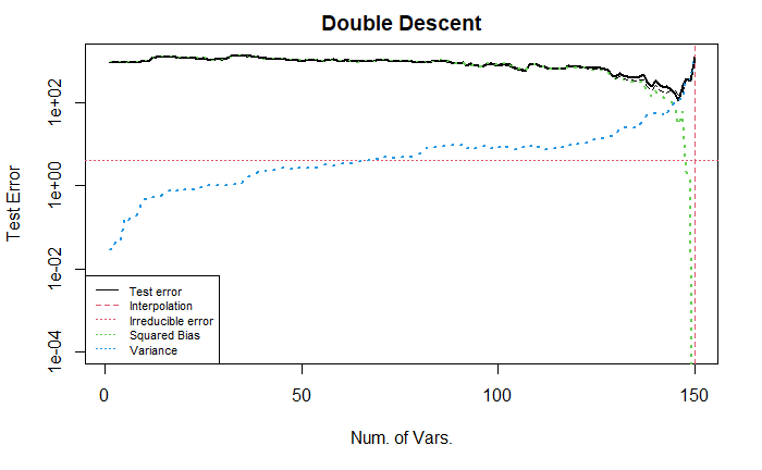
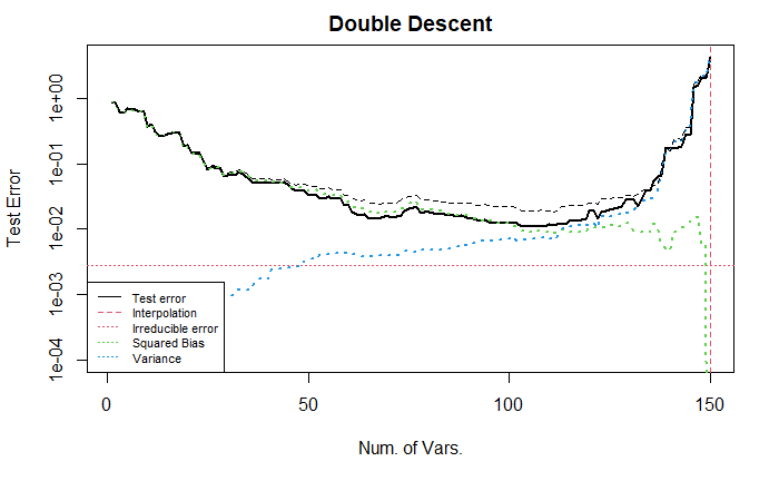
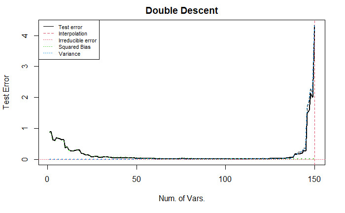
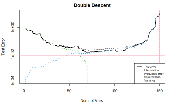
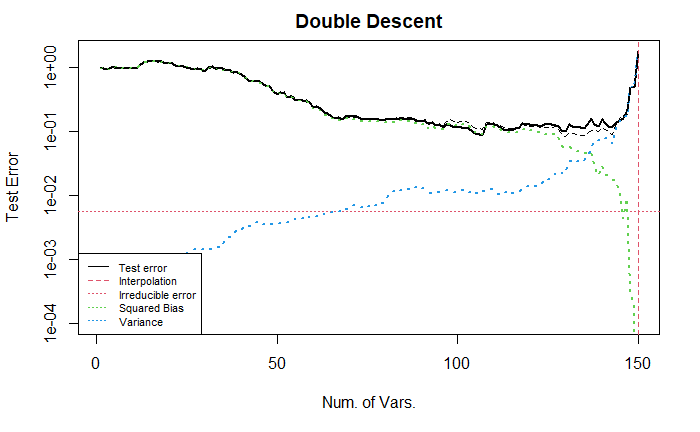
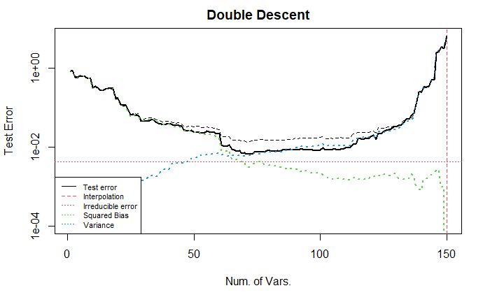
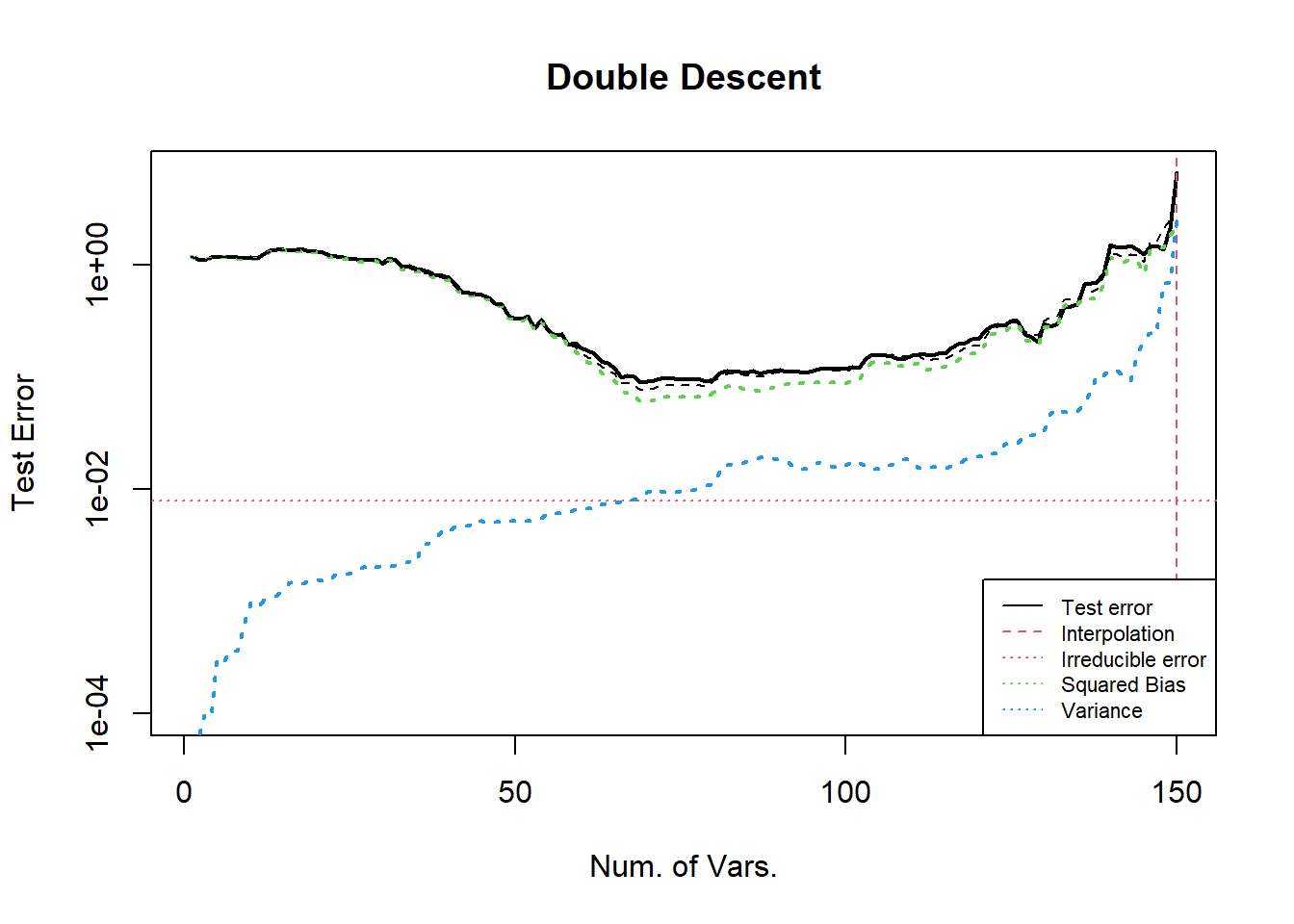
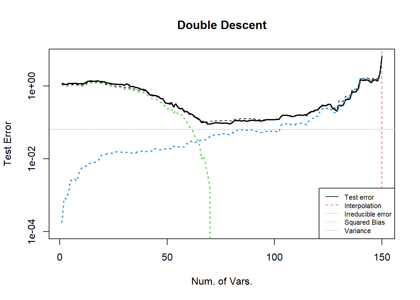
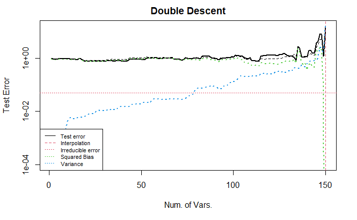
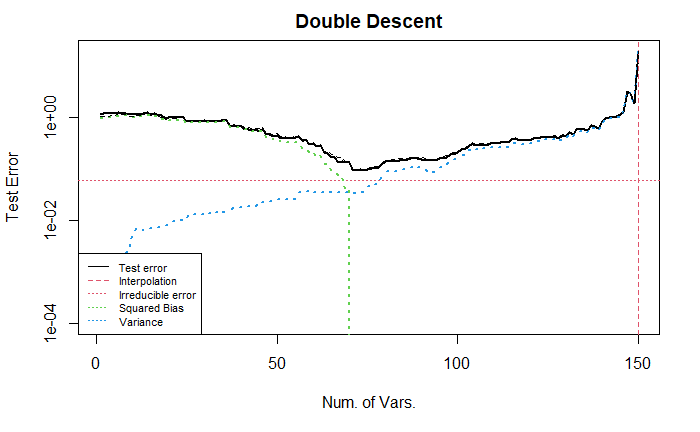
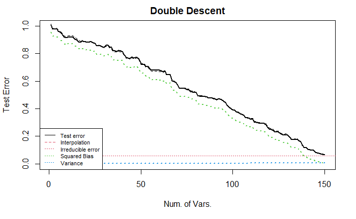
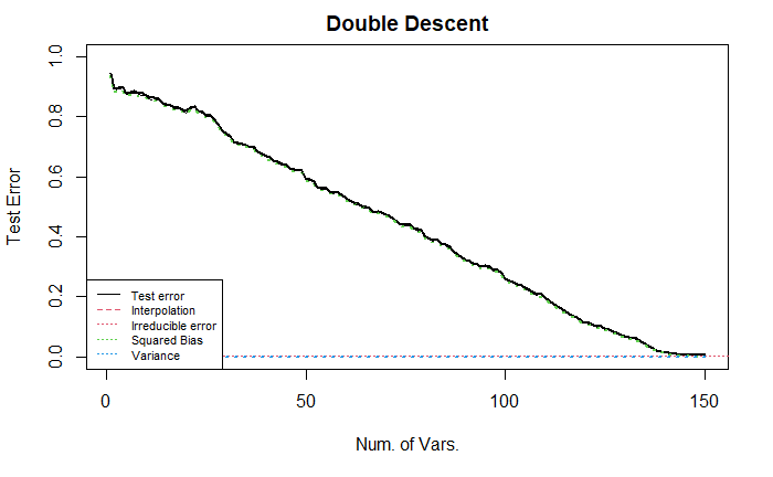
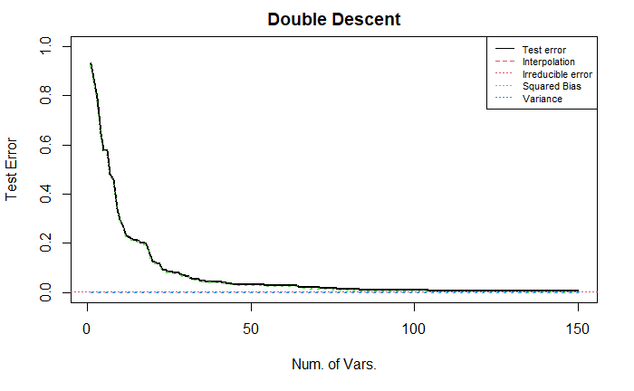
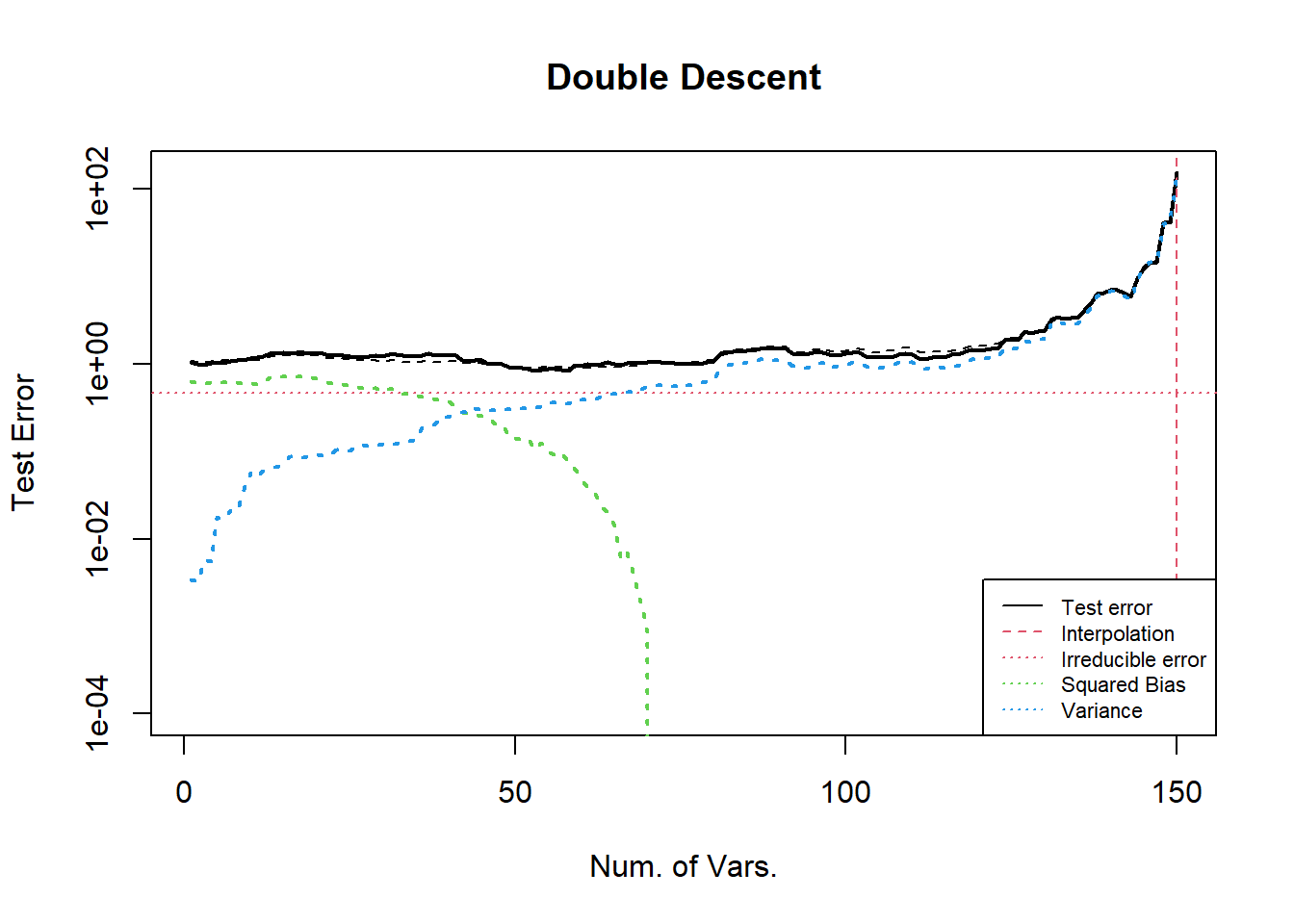
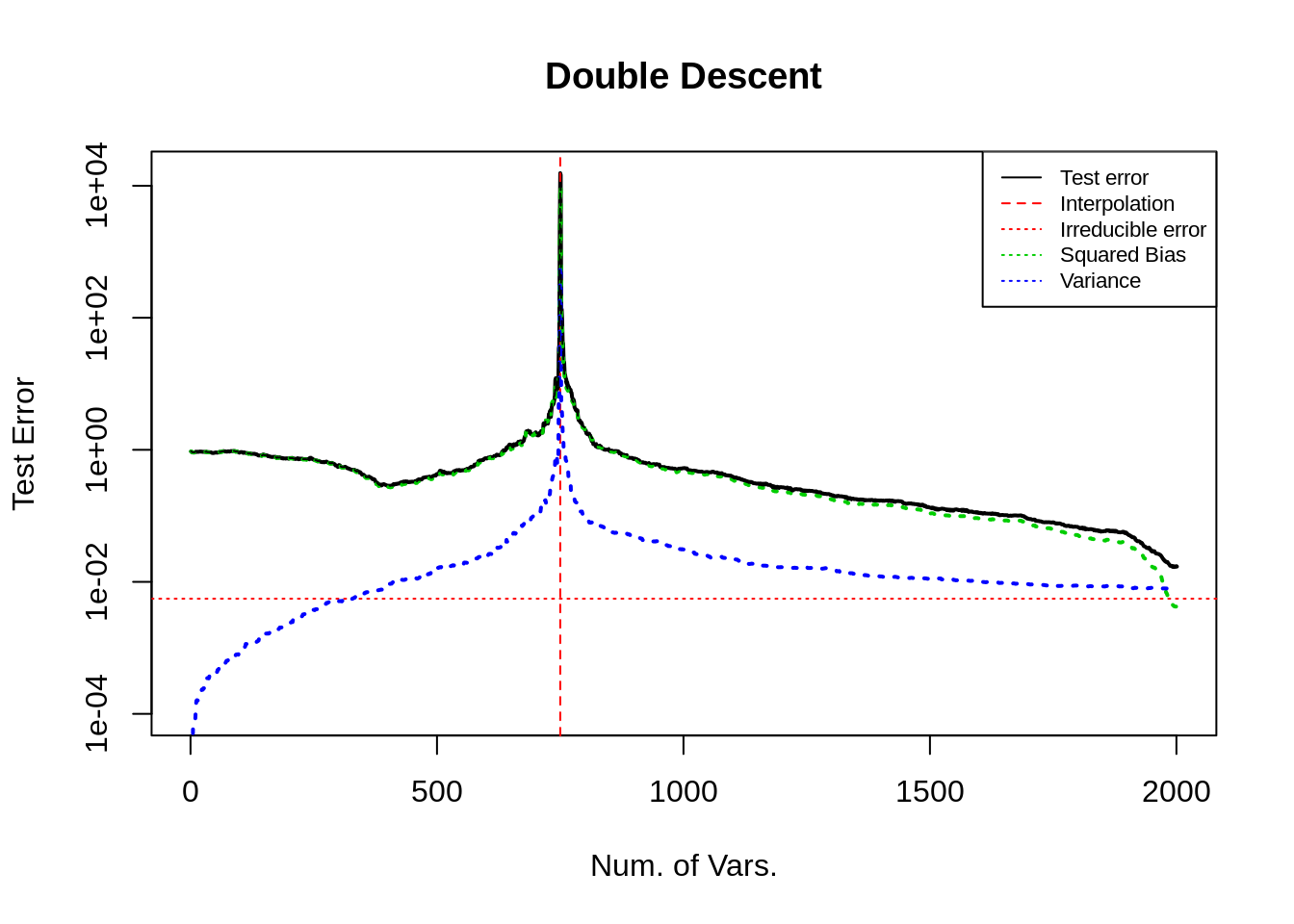
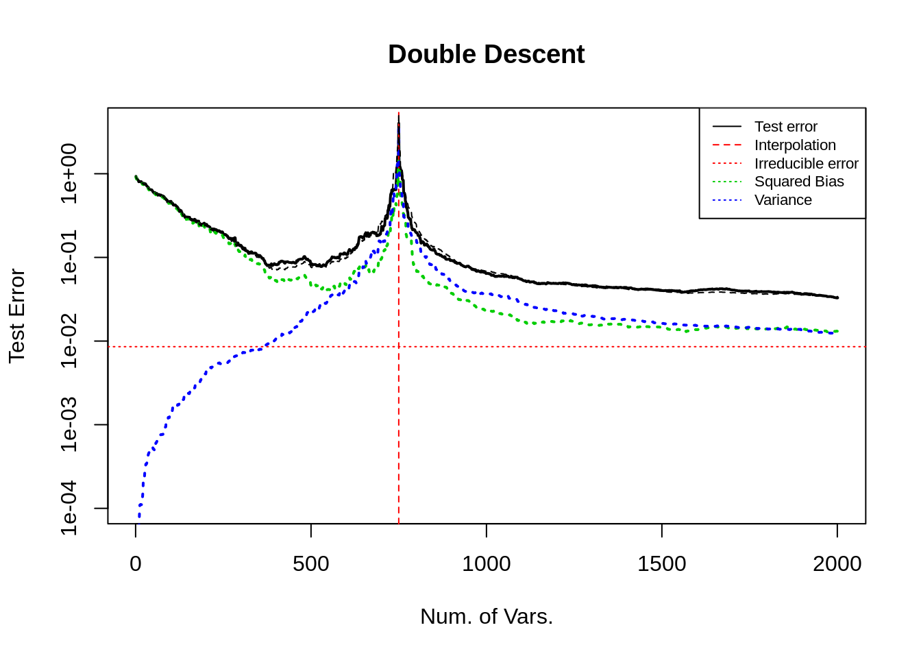
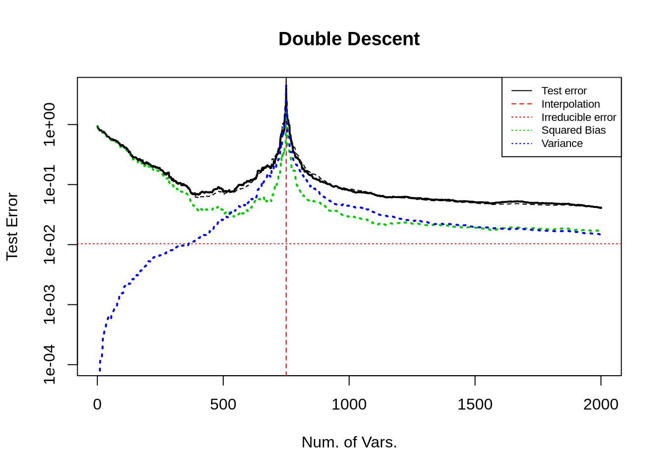
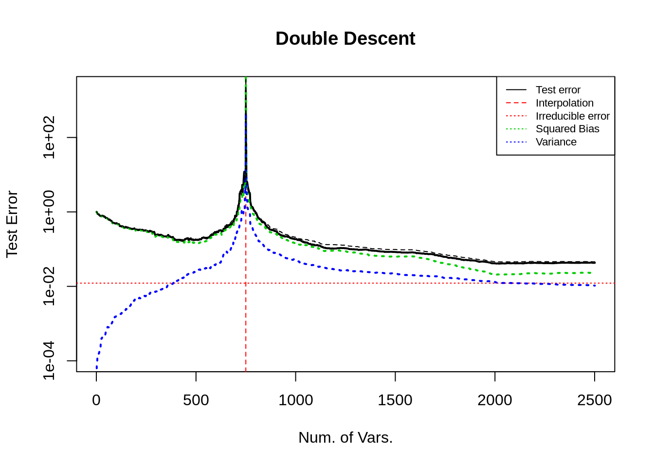
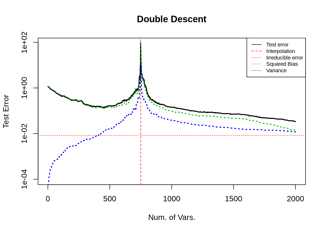
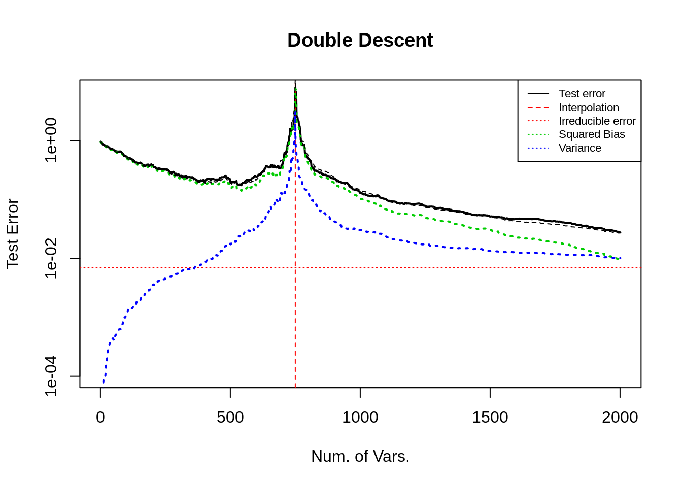
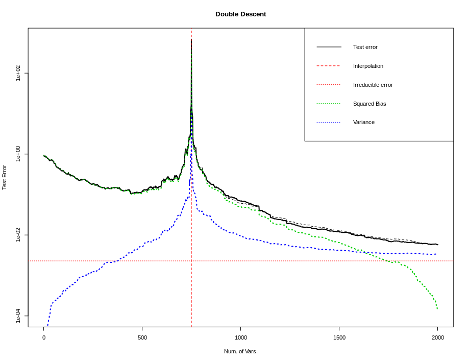
<p>Consider here the influence of different simulation settings on the double falling curve. The images show the test error (black solid line), squared bias term (green dotted line), variance term (blue dotted line), irreducible error term (red horizontal dashed line), the sum of squared bias variance and  irreducible error (black dotted line, almost coincides with the test error), interpolation point (red vertical dotted line).</p>

<p>\(\mathbf{x}\sim N(\mu, \Sigma)\), 抽样 \(n\) 次, 其中 \(75\%\) 用于训练, 剩余的样本用于测试, \(\mu\) 的取值在后文讨论, 协方差矩阵 \(\Sigma\) 设置为自回归形式, 即 \(\Sigma_{i,j} = \rho^{\vert i-j \vert}\), \(\rho\) 的取值在后文讨论.</p>

<p>The expected test error can be decomposed as the sum of irreducible error, squared bias term and variance term.</p>

<p>Bias term: \(\sum_{i\in \text{Test}} (X_i \hat{\boldsymbol{\beta}}_0 - Y_0)^2\); 它与样本量与预测性能有关, 样本越多, 它越准则 (波动越小); 预测值与 (未知) 真实值越接近, 它越小. OLS 框架下, 它表示回归时遗漏信号的大小 (各协变量的样本方差乘以参数的平方之和).</p>

<p>Variance term: \(\sum_{i\in \text{Test}} (X_i \hat{\boldsymbol{\beta}} - X_i \hat{\boldsymbol{\beta}}_0)^2\); 它与样本量以及参数个数有关, 样本量越大它越小, 变量越多它越大. 在 OLS 框架下有具体地分析. 方差项的理论值在已知 \(Y_0\) 时可以具体计算.</p>

<p>irreducible error: \(\sum_{i\in \text{Test}} (X_i \hat{\boldsymbol{\beta}}_0 - Y_i)^2\); 它与样本量有关, 当样本量足够大时, 它趋向于随机误差的方差.</p>

<p>且为了凸显曲线的形状, 使曲线更加平滑, (如无额外说明) 图的纵坐标都使用对数轴. 后文对此进行了讨论.</p>

<p>We load the following packages in our code.</p>

<div class="language-R highlighter-rouge"><div class="highlight"><pre class="highlight"><code><span class="n">library</span><span class="p">(</span><span class="n">MASS</span><span class="p">)</span><span class="w">     </span><span class="c1"># for mvrnorm()</span><span class="w">
</span><span class="n">library</span><span class="p">(</span><span class="n">parallel</span><span class="p">)</span><span class="w"> </span><span class="c1"># for detectCores()</span><span class="w">
</span></code></pre></div></div>

<h2 id="2-u-curve">2. U curve</h2>
<p>在线性模型的设定中, 增加变量数量, 观察 U 型曲线, 根据误差的分解, 研究是什么因素导致了测试误差的 U 型.</p>

<h3 id="q--a">Q &amp; A</h3>

<ul>
  <li><strong>bias 是否会随着变量的增加而增加?</strong></li>
</ul>

<blockquote>
  <p>答: 会, 这与传统的 bias-variance trade-off 相左.</p>

  <p>例子: 如 Case 1, 2 图, 如果不遗漏变量, bias 在末尾下降至 0. 而 Case 4 中遗漏了模型中的非零变量, bias在后半段不仅不降低, 反而增加了.</p>
</blockquote>

<p>解释: 由于 bias 项受到样本量以及预测性能的影响. (预测性能/能力, 解释为在无限多样本的情况下, 预测方法的最佳表现.) 
一方面, 虽然在变量逐渐都纳入回归时, 预测性能逐渐趋于 (回归方法的) 最佳. 注意到, 此时最佳参数并不能最小化训练误差. 
另一方面, 样本量也影响了 bias 项, 在样本量略微大于变量数时, (特别是遗漏了非零变量的插值时) 回归方法 (OLSE) 可以利用任何变量解释训练数据. 事实上, 插值点之前, 由于变量增多, 变量张成的空间也增大, 因此可以持续地降低训练误差, 但为这些变量分配的错误的系数会反向增大测试误差 (模型越来越差); 且在插值时训练误差必然为 0, 而测试误差达到最大. 
因此从观测值中得到一个远离真实模型的过拟合的模型, 使得出现了模型越来越好但是 bias 反而越来越大的情况. 但是当模型没有遗漏非零变量时, 正确的系数恰好对应了最好的插值, 此时偏差为 0. (可以参考 3.3 节对样本的讨论, 只要有足够多的样本, 偏差可以保持非增, 即使不降低至 0.)
这一点可以通过观察 \(\|\hat{\boldsymbol{\beta}}\|_2\) 有更加直观的理解.</p>

<ul>
  <li><strong>为什么方差递增, 在插值处加速达到峰值?</strong></li>
</ul>

<blockquote>
  <p>答: OLS 框架可以解释方差递增问题, 但是 (错误的) 过拟合才能解释峰值.</p>
</blockquote>

<p>解释: OLS 框架下讨论过估计量的方差, 为 \(\sigma^2 p/n\); 但这只能解释前半段, 样本充足时方差缓慢增长的趋势. 但是接近插值点时, 方差快速且剧烈地增长. 这个现象, 直观上, 我认为是样本数过于接近变量数, LSE 更偏向于插值而不是回归, 此时系数的估计量失真, 远远地偏离正确值, 造成预测值也产生了较大的偏差.  更具体地, 系数估计值的误差为 \((X^TX)^{-1}X^T \epsilon\), 这一项本来由于 \(\epsilon\) 与 \(\mathbf{x}\) 的独立性, 是接近于 0 的, 但在插值时, 随机误差可以被变量 (错误地) 解释, 即增加了估计量的范数, 从而增加了预测值的大小. 更严格地推理需要从数学上下手, 可以通过分析 \(\|X_{test} (X^TX)^{-1}X^T \epsilon\|_2\) 得知具体的情况.</p>

<h3 id="21-tuning-coefficients-boldsymbolbeta--of-mathbfx">2.1 Tuning coefficients \(\boldsymbol{\beta}\)  of \(\mathbf{x}\)</h3>
<h4 id="case-1-all-elements-in-boldsymbolbeta_0-are-non-zero">Case 1: All elements in \(\boldsymbol{\beta}_0\) are non-zero</h4>
<p>200 个样本, 150个变量. 每个变量都赋予了随机的非零系数 (采样于均值为二项分布且方差为1的正态分布).</p>

<p><img src="../assets/202101081519281.png" alt="image" style="zoom:90%;" /></p>

<p>从图中可以看出, 当变量从 1 增大到 120 时, 测试误差基本不变, 其中方差不断增加, 偏差基本保持不变, 此时方差项对测试误差的影响较小可以忽略不记; 
当变量继续增大, 方差维持相同的趋势增长, 但偏差迅速下降, 导致测试误差先下降再上升, 呈现 U 型.</p>

<p>由于随机性的影响, 测试误差或bias在变量数为 1–120 时的 (几乎) 水平趋势. 如样本量充足, 试误差或 bias 将规律地递减.</p>

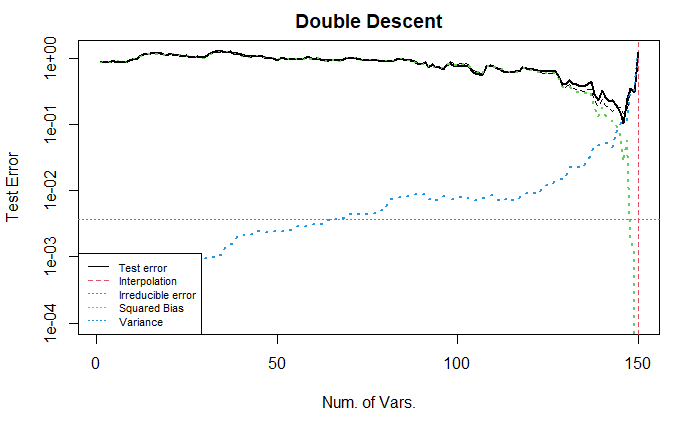
<p>下面, 我们将数据 \(Y\) 进行了标准化, 让误差曲线的范围 (大致) 在 \([0,1]\) 之间.</p>

<p><img src="../assets/202101081519291.png" alt="image" style="zoom:90%;" /></p>

<p>如图所示, 曲线与不标准化的曲线完全一致, 只是坐标轴不同, 导致一些尺度不同. 
该设置模仿了 <a href="https://arxiv.org/abs/1812.11118v2">Belkin et al. 2018</a>.</p>

<p>下面, 我们将协变量的顺序进行了随机排序, 保留了对 \(Y\) 的标准化 (即对系数的标准化). (由于采用的是自回归形式的协方差, 因此邻近变量的相关性强, 距离较远的协变量相关性较弱. 这会影响bias曲线的变化过程).</p>

<p><img src="../assets/20210108151930.png" alt="image" style="zoom:90%;" /></p>

<p>上图展示了较为标准的 U 型曲线. 
<strong>我不清楚为什么经过随机排序后的误差曲线会展现出 U 型</strong>. 
直观上, 由于我们在回归时逐个增加变量, 变量的排序会影响回归的效果, 例如按照系数大小排序或者随机排序的结果显然是不同的.</p>

<p>同时, 要注意到上面展示的都是对数变换后的纵轴, 实际的 (未经过对数变换) 测试误差曲线更加陡峭, 如下所示.</p>

<p><img src="../assets/20210108151931.png" alt="image" style="zoom:90%;" /></p>

<h4 id="case-2-special-boldsymbolbeta_0">Case 2: Special \(\boldsymbol{\beta}_0\)</h4>
<p>与上面的情况形成对比, 在这里, 我们设置非零的系数出现在较前的变量中 (1–70), 而靠后的变量都是冗余变量 (系数为0).</p>

<p>偏差曲线随着变量个数得增加而持续下降, 当变量数为 70 时, 所有真实的变量都被纳入回归, 此后的偏差项保持为 0 不变. 
该图依然显示出了测试误差的 U 型.</p>

<p><img src="../assets/20210108151932.png" alt="image" style="zoom:90%;" /></p>

<h4 id="case-3-special-boldsymbolbeta_0">Case 3: Special \(\boldsymbol{\beta}_0\)</h4>

<p>与上面的情况形成对比, 考虑所有系数都非零, 但将前半部分 (1–70) 系数增大, 此时不调整 x 的顺序.</p>

<p>从图中可以看出, 变量个数在 25–70 时, 测试误差逐渐下降; 70–120 时, 稳定; 之后加速下降到 0.</p>

<p><img src="../assets/20210108151935.png" alt="image" style="zoom:90%;" /></p>

<p>下图展示了调整 x 的顺序后的结果. 
需要注意到, 当变量个数大于 70 时, bias 下降缓慢. (小的系数对应的变量被纳入回归带来的小幅度的变化在前面的例子中可能也存在, 但是由于比例太小, 在图中无法显示出来)</p>

<p><img src="../assets/202101081519292.png" alt="image" style="zoom:90%;" /></p>

<h4 id="case-4-misspecified-model">Case 4: Misspecified model</h4>

<p>这里我们从另一个角度来考虑模型的设定, 将随机误差视为未纳入模型的非零变量. (参考 Q &amp; A 1)</p>

<p>下面我们考虑所有模型都是误设定的情况, 即在回归中忽略一些非零变量, 此时可以预计 bias 曲线不会下降到 0 而是下降到某个定值. 
注意, 模型误设定等价于将没有考虑的变量与随机误差项合并, 这里的改动等价于修改了随机误差. 测试误差 / 方差曲线并不会变动. 
但是由于正确模型是已知的, 因此 bias 曲线会变动. 即偏差与方差之和 (黑色虚线) 会变动.</p>

<p><img src="../assets/2021010815292.png" alt="image" style="zoom:46%;" /></p>

<p>下图展示的是将引入的信息放在随机误差项中的情况.</p>

<p><img src="../assets/2021010815293.png" alt="image" style="zoom:46%;" /></p>

<p>可以发现, 偏差项在纳入了所有正确变量之后, 降低到了 0; 同时相比于上一个例子 irreducible error 增加了; 方差曲线没有变化.</p>

<h3 id="22-tuning-covariance-sigma-of-mathbfx">2.2 Tuning covariance \(\Sigma\) of \(\mathbf{x}\)</h3>
<p>与上面的例子不同的是, 这里将变量间的相关系数调低. 
首先考虑所有系数都非零的情况, 可以从图中看到, 类似于自回归结构的协方差矩阵的结果, 当几乎所有变量都被纳入回归后, 偏差才(急速)下降.</p>

<p><img src="../assets/20210108151933.png" alt="image" style="zoom:90%;" /></p>

<p>接着, 我们考虑第二种系数设定(后半部分全为零).</p>

<p><img src="../assets/20210108151934.png" alt="image" style="zoom:90%;" /></p>

<h3 id="23-tuning-sample-size">2.3 Tuning sample size</h3>

<p>这里, 将独立样本以及 Case 1 的系数的设置略作修改, 样本个数从 200 调整为 2000, 可以去掉部分随机性, 同时凸显出变化的本质. 
由于变量个数依旧为 150, 没有改变, 因此下面的图中都没有出现 U 型, 而是单调递减的直线/曲线.</p>

<p><em>注意, 这一部分的纵坐标不做对数变换. (因为我希望直观的观察每个变量对测试误差的影响)</em></p>

<p><img src="../assets/202101081519293.png" alt="image" style="zoom:90%;" /></p>

<p>上图中, 绿线线性地递减, 告诉我们, 每个非零变量被纳入回归中, 都会带来测试误差的降低, 并且样本量充足时, 偏差可以降低到 0. 
蓝线几乎水平, 表明当样本足够多时, 方差项几乎不变.</p>

<p>下面, 我们将样本的相关性增加 (参数为 0.9 的自回归结构).</p>

<p><img src="../assets/202101081519294.png" alt="image" style="zoom:90%;" /></p>

<p>该图中的偏差项与上图类似; 而方差项降低了, 始终保持 0, 即样本的增加让每个线性回归得到的系数与拟真的系数之间的距离减小了.</p>

<p>下面, 我们在上述的基础上, 将样本随机排序 (样本独立时, 不需要进行随机排序, 因为排序之后的样本协方差结构不变, 结果显然不变. 但是样本不独立时, 结果如下.)</p>

<p><img src="../assets/202101081519295.png" alt="image" style="zoom:90%;" /></p>

<p>该图展现出前半部分的变量对测试误差的下降有巨大的贡献, 但后半部分的变量对测试误差几乎没有影响(有, 但是较小).</p>

<p>我认为, 这是因为样本随机排序之后, 相邻变量之间的相关性不高, 但是远距离变量之间的相关性却有可能很高 (0.9), 因此, 在前半段的变量中, 可能某些变量并不是非零变量 (而是冗余变量), 但由于它可能与某些非零变量高度相关, 因此在回归中包含了部分由于这种相关性带来的信息, 导致测试误差下降. 
同时, 当它对应的真实非零变量被纳入回归中时, 真实变量具有比冗余变量更多的信息, 因此可以让测试误差继续 (小幅度地) 下降. 
因此, 随着变量个数的增加, 越来越少的信息被新纳入回归模型中, 即对应了测试误差曲线的导数越来越接近 0.</p>

<h3 id="24-tuning-random-error-epsilon">2.4 Tuning random error \(\epsilon\)</h3>

<p>这里我们使用 3.1 节中的 Case 2 来设置系数, 考虑增大随机误差项 (方差扩大 10 倍), 参考 3.1 节 Case 4, 这种调整等价于调整模型的设定, 让回归忽略更多的有效变量.</p>

<p><img src="../assets/2021010815294.png" alt="image" style="zoom:46%;" /></p>

<p>可以发现, 方差项在插值点处具有更高的峰值 (差不多也是 10 倍).</p>

<h3 id="25-summary-and-code">2.5 Summary and Code</h3>

<p>上述部分调整了样本大小 n, 变量 x 的协方差结构, 变量系数的结构. 
所有调整都可以通过下面的代码实现.</p>

<div class="language-R highlighter-rouge"><div class="highlight"><pre class="highlight"><code><span class="n">set.seed</span><span class="p">(</span><span class="m">1111</span><span class="p">)</span><span class="w">
</span><span class="c1">## settings</span><span class="w">
</span><span class="n">n</span><span class="w"> </span><span class="o">&lt;-</span><span class="w"> </span><span class="m">200</span><span class="w">  </span><span class="c1"># default: 200; special: 2000</span><span class="w">
</span><span class="n">p</span><span class="w"> </span><span class="o">&lt;-</span><span class="w"> </span><span class="m">149</span><span class="w">  </span><span class="c1"># default: 149;</span><span class="w">
</span><span class="n">n_train</span><span class="w"> </span><span class="o">&lt;-</span><span class="w"> </span><span class="nf">as.integer</span><span class="p">(</span><span class="n">n</span><span class="w"> </span><span class="o">*</span><span class="w"> </span><span class="m">0.75</span><span class="p">)</span><span class="w">
</span><span class="n">n_test</span><span class="w"> </span><span class="o">&lt;-</span><span class="w"> </span><span class="n">n</span><span class="w"> </span><span class="o">-</span><span class="w"> </span><span class="n">n_train</span><span class="w">
</span><span class="c1"># model settings</span><span class="w">
</span><span class="n">mean_x</span><span class="w"> </span><span class="o">&lt;-</span><span class="w"> </span><span class="nf">c</span><span class="p">(</span><span class="nf">rep</span><span class="p">(</span><span class="m">0</span><span class="p">,</span><span class="n">p</span><span class="p">))</span><span class="w">
</span><span class="n">sigma_x</span><span class="w"> </span><span class="o">&lt;-</span><span class="w"> </span><span class="n">matrix</span><span class="p">(</span><span class="m">0</span><span class="p">,</span><span class="n">p</span><span class="p">,</span><span class="n">p</span><span class="p">)</span><span class="w">     
</span><span class="k">for</span><span class="w"> </span><span class="p">(</span><span class="n">i</span><span class="w"> </span><span class="k">in</span><span class="w"> </span><span class="m">1</span><span class="o">:</span><span class="n">p</span><span class="p">){</span><span class="w">
  </span><span class="k">for</span><span class="w"> </span><span class="p">(</span><span class="n">j</span><span class="w"> </span><span class="k">in</span><span class="w"> </span><span class="m">1</span><span class="o">:</span><span class="n">p</span><span class="p">){</span><span class="w">
    </span><span class="n">sigma_x</span><span class="p">[</span><span class="n">i</span><span class="p">,</span><span class="n">j</span><span class="p">]</span><span class="w"> </span><span class="o">&lt;-</span><span class="w"> </span><span class="m">0.9</span><span class="o">^</span><span class="nf">abs</span><span class="p">(</span><span class="n">i</span><span class="o">-</span><span class="n">j</span><span class="p">)</span><span class="w">      </span><span class="c1"># 0.01 0.9</span><span class="w">
  </span><span class="p">}</span><span class="w">
</span><span class="p">}</span><span class="w">
</span><span class="n">mean_e</span><span class="w"> </span><span class="o">&lt;-</span><span class="w"> </span><span class="nf">c</span><span class="p">(</span><span class="nf">rep</span><span class="p">(</span><span class="m">0</span><span class="p">,</span><span class="n">n</span><span class="p">))</span><span class="w">
</span><span class="n">sigma_e</span><span class="w"> </span><span class="o">&lt;-</span><span class="w"> </span><span class="n">diag</span><span class="p">(</span><span class="n">x</span><span class="o">=</span><span class="m">1</span><span class="p">,</span><span class="n">n</span><span class="p">,</span><span class="n">n</span><span class="p">)</span><span class="w">
</span><span class="n">x</span><span class="w"> </span><span class="o">&lt;-</span><span class="w"> </span><span class="n">mvrnorm</span><span class="p">(</span><span class="n">n</span><span class="o">=</span><span class="n">n</span><span class="p">,</span><span class="n">mean_x</span><span class="p">,</span><span class="n">sigma_x</span><span class="p">)</span><span class="w">
</span><span class="c1">#x &lt;- x[, sample(p)]                  # Random sorting columns of x</span><span class="w">
</span><span class="n">e</span><span class="w"> </span><span class="o">&lt;-</span><span class="w"> </span><span class="n">mvrnorm</span><span class="p">(</span><span class="n">n</span><span class="o">=</span><span class="m">1</span><span class="p">,</span><span class="n">mean_e</span><span class="p">,</span><span class="n">sigma_e</span><span class="p">)</span><span class="w"> </span><span class="o">*</span><span class="w"> </span><span class="m">2</span><span class="w">  </span><span class="c1"># variance of random error 2</span><span class="w">
</span><span class="n">beta0</span><span class="w"> </span><span class="o">&lt;-</span><span class="w"> </span><span class="nf">c</span><span class="p">(</span><span class="nf">rep</span><span class="p">(</span><span class="m">0</span><span class="p">,</span><span class="n">p</span><span class="p">))</span><span class="w">

</span><span class="c1">### setting beta0</span><span class="w">
</span><span class="c1">## Case 1</span><span class="w">
</span><span class="n">mean_beta</span><span class="w"> </span><span class="o">&lt;-</span><span class="w"> </span><span class="n">rbinom</span><span class="p">(</span><span class="n">p</span><span class="p">,</span><span class="w"> </span><span class="m">10</span><span class="p">,</span><span class="w"> </span><span class="m">0.3</span><span class="p">)</span><span class="w"> </span><span class="o">*</span><span class="w"> </span><span class="m">4</span><span class="w">
</span><span class="n">beta0</span><span class="w"> </span><span class="o">&lt;-</span><span class="w"> </span><span class="n">mvrnorm</span><span class="p">(</span><span class="n">n</span><span class="o">=</span><span class="m">1</span><span class="p">,</span><span class="w"> </span><span class="n">mean_beta</span><span class="p">,</span><span class="w"> </span><span class="n">diag</span><span class="p">(</span><span class="n">p</span><span class="p">))</span><span class="w">
</span><span class="n">beta0</span><span class="p">[</span><span class="n">which</span><span class="p">(</span><span class="nf">abs</span><span class="p">(</span><span class="n">beta0</span><span class="p">)</span><span class="w"> </span><span class="o">&lt;</span><span class="w"> </span><span class="m">1e-1</span><span class="p">)]</span><span class="w"> </span><span class="o">&lt;-</span><span class="w"> </span><span class="m">0</span><span class="w">
</span><span class="c1">## Case 2</span><span class="w">
</span><span class="c1"># beta0[(1:35)*2] &lt;- rep(40, 35)</span><span class="w">
</span><span class="c1">## Case 3</span><span class="w">
</span><span class="c1"># mean_beta &lt;- rbinom(p, 10, 0.3) * 4</span><span class="w">
</span><span class="c1"># beta0 &lt;- mvrnorm(n=1, mean_beta, diag(p))</span><span class="w">
</span><span class="c1"># beta0[(1:35)*2] &lt;- rep(80, 35)</span><span class="w">
</span><span class="c1"># beta0[which(abs(beta0) &lt; 1e-1)] &lt;- 0</span><span class="w">
</span><span class="n">beta0</span><span class="w"> </span><span class="o">&lt;-</span><span class="w"> </span><span class="n">beta0</span><span class="w"> </span><span class="o">/</span><span class="w"> </span><span class="n">norm</span><span class="p">(</span><span class="n">beta0</span><span class="p">,</span><span class="n">type</span><span class="o">=</span><span class="s2">"2"</span><span class="p">)</span><span class="w"> </span><span class="o">*</span><span class="w"> </span><span class="m">8</span><span class="w">   </span><span class="c1"># control SNR</span><span class="w">

</span><span class="c1"># linear model (corrected / mis-specificted model)</span><span class="w">
</span><span class="n">y0</span><span class="w"> </span><span class="o">&lt;-</span><span class="w"> </span><span class="n">x</span><span class="w"> </span><span class="o">%*%</span><span class="w"> </span><span class="n">beta0</span><span class="w"> </span><span class="o">+</span><span class="w"> </span><span class="n">mvrnorm</span><span class="p">(</span><span class="n">n</span><span class="o">=</span><span class="n">n</span><span class="p">,</span><span class="nf">rep</span><span class="p">(</span><span class="m">0</span><span class="p">,</span><span class="m">20</span><span class="p">),</span><span class="n">diag</span><span class="p">(</span><span class="m">20</span><span class="p">))</span><span class="w"> </span><span class="o">%*%</span><span class="w"> </span><span class="nf">rep</span><span class="p">(</span><span class="m">0.5</span><span class="p">,</span><span class="m">20</span><span class="p">)</span><span class="w">
</span><span class="n">y</span><span class="w"> </span><span class="o">&lt;-</span><span class="w"> </span><span class="n">y0</span><span class="w"> </span><span class="o">+</span><span class="w"> </span><span class="n">e</span><span class="w"> </span><span class="c1"># * 10</span><span class="w">
</span><span class="c1">## some standardization</span><span class="w">
</span><span class="n">beta0</span><span class="w"> </span><span class="o">&lt;-</span><span class="w"> </span><span class="n">beta0</span><span class="w"> </span><span class="o">/</span><span class="w"> </span><span class="n">sd</span><span class="p">(</span><span class="n">y</span><span class="p">)</span><span class="w">
</span><span class="n">y0</span><span class="w"> </span><span class="o">&lt;-</span><span class="w"> </span><span class="n">y0</span><span class="w"> </span><span class="o">/</span><span class="w"> </span><span class="n">sd</span><span class="p">(</span><span class="n">y</span><span class="p">)</span><span class="w">
</span><span class="n">y</span><span class="w"> </span><span class="o">&lt;-</span><span class="w"> </span><span class="n">y</span><span class="w"> </span><span class="o">/</span><span class="w"> </span><span class="n">sd</span><span class="p">(</span><span class="n">y</span><span class="p">)</span><span class="w">
</span></code></pre></div></div>

<h2 id="3-double-descent-curve">3. Double descent curve</h2>

<p>要展示双下降, 我们在 U curve 的基础上, 增加 (与模型变量相关的) 变量的个数.</p>

<p>可以操控的因素与 U curve 中提及的类似. 下面我们讨论不同因素对曲线的影响. 以及如何才能展示出较完美的双下降曲线.</p>

<h3 id="q--a-1">Q &amp; A</h3>

<ul>
  <li><strong>为什么在插值点之后, 增加变量会降低偏差?</strong></li>
</ul>

<p>答: 由于估计方法的压缩效应.</p>

<p>解释: 插值点之后的预测值都是对训练样本的插值. 但是不同的插值也可以区分优劣, 最好的插值是: 容纳了所有的非零变量的插值, 但 它仅仅有较小的范数, 而未必具有最小的范数. 在变量增加的初期, 由于估计量的压缩效应, 预测方法会寻找范数较小的系数估计, 当变量继续增加的时候, 能够找到的插值方式也同步增加, 此时的系数估计越来越好, 从而测试误差也越来越小. 
(继续增加可以发现估计得到的系数的范数低于真实系数的范数. 这可能是由于真实模型中非零变量太多. )</p>

<ul>
  <li><strong>为什么在插值点之后,  增加变量会降低方差? 会降低到哪儿?</strong></li>
</ul>

<p>答: 与奇异向量的分布有关, 会缓慢 (越来越慢) 降至 0.</p>

<p>解释: 由于测试误差可以写成 \(\left\|X_{test} V\begin{pmatrix}D_1^{-1} \\ \mathbf{0}_{p-n,n}\end{pmatrix} U^T \epsilon\right\|_2\). 对于任意一个测试样本, 记为 \(X_{t}\in\mathbb{R}^{p\times 1}\), 考虑它的测试误差. 即 \(X_{t}^T V\begin{pmatrix}D_1^{-1} \\ \mathbf{0}_{p-n,n}\end{pmatrix} U^T \epsilon\). 
这里只考虑它的上界, 由 Cauchy 不等式可知, 它小于 \(\left\|X_{t}^T \begin{pmatrix}D_1^{-1} \\ \mathbf{0}_{p-n,n}\end{pmatrix}\right\|_2 \|\epsilon\|_2\). 
可以知道, 该上界是随着 \(p\) 的增加而减少的. 
更严格的证明我还没有想到.</p>

<h3 id="31-tuning-coefficients-boldsymbolbeta--of-mathbfx">3.1 Tuning coefficients \(\boldsymbol{\beta}\)  of \(\mathbf{x}\)</h3>

<h4 id="case-1-base">Case 1: Base</h4>
<p>这个实验的效果比较好,可以展示双下降的现象. 
考虑线性模型中的不同参数的设置情况.</p>

<p>样本量 1000, 变量个数 2000, 使用参数为 0.9 的自相关结构的协方差矩阵生成正态分布的 i.i.d. 变量. 
模型为线性, 变量的系数类似与 U curve 中描述的设置方法, 具体地, 第 1–400 个变量系数都为 40, 其他的系数从独立的且均值为 Binomial(10, 0.1), 方差为 1 的正态分布中采样, 最后将与 0 的距离小于 \(10^{-3}\) 的系数设置为 0 (作用不大, 但形式上具有一定的稀疏性). 最后调整向量的 2 范数 (控制信噪比).</p>

<p><img src="../assets/202101081519296.png" alt="image" style="zoom:46%;" /></p>

<p>从图中可以看出, 测试误差呈现出了双下降的趋势. 
在插值点 (红色垂直虚线) 左侧, 误差先下降后上升为 U 型, 机理与前文 U curve 3.4 节所述的相同, 且在插值点处的测试误差远大于 \(Y\) 的方差. 方差项一直增大, 但从绝对大小上看, 相对于偏差项较小, 可忽略. 偏差项于主导了测试误差项的变化.</p>

<p>下面, 我们调整变量的顺序为随机排序.</p>

<p><img src="../assets/202101081519297.png" alt="image" style="zoom:46%;" /></p>

<p>上图, 测试误差曲线更加平顺, U 型部分前半段下降得更快一些 (理由如 U curve 中所述).</p>

<p>下面, 在上述基础上, 我将第 500–1000 的变量系数设置成 0.</p>

<p><img src="../assets/2021010815290.png" alt="image" style="zoom:46%;" /></p>

<p>经过仔细核对, 这种设置对册数误差曲线几乎没有影响.</p>

<h4 id="case-2-增加冗余变量">Case 2: 增加冗余变量</h4>

<p>这里, 我增加了 500 个冗余变量于末尾, 其他设定不变. 观察变化.</p>

<p><strong>这张图的随机数种子与上面的不同, 因此曲线有些不同, 可以修改一下随机数</strong></p>

<p><img src="../assets/202101081519299.png" alt="image" style="zoom:46%;" /></p>

<p>上图表示出, 在 \(p&gt;n\) (且远离插值点) 时, 增加无用的变量不会改变偏差, 方差几乎不变, 总的来看, 测试误差几乎不改变. 
这提醒我, 如果要降低偏差曲线, 必须要考虑增加有用的变量, 而不是无用的变量.</p>

<p><strong>这与 U 型曲线中的现象可能不一致, 需要考虑在 U curve 的实验中也在末尾增加无用的变量, 观察偏差和方差的变化</strong>, 我预计, 偏差不变但是方差会改变.</p>

<h4 id="case-3-增大尾部系数的大小">Case 3: 增大尾部系数的大小</h4>

<p>在 base 模型的基础上, 将末尾的 200 个变量对应的系数增大, 且令中间峰值部分的系数为 0 , 最终留下约 1500 个非零系数; 变量随机排序. 
其他设置同前.</p>

<p><img src="../assets/202101081519298.png" alt="image" style="zoom:46%;" /></p>

<p>可以让 bias 曲线的尾部下降得更快. 
(这是符合逻辑的结果, 因为 bias 会在重要(大系数)变量纳入模型时下降. 见 U curve 部分. )</p>

<h4 id="case-4-减小首部系数的大小">Case 4: 减小首部系数的大小</h4>

<p>在 base 模型的基础上, 我们将开始的 200 个变量对应的系数减小. (base是增大后的结果, 从代码中删去部分行既可. )</p>

<p><img src="../assets/2021010815291.png" alt="image" style="zoom:46%;" /></p>

<p>从图中可以看出, 这种设置不改变曲线的走势.</p>

<h4 id="case-5-寻找-bias-的极值">Case 5: 寻找 bias 的极值</h4>

<p>寻找 bias 的最大值可以, 参考 U curve 中 Q &amp; A 以及 Case 4 的结果.</p>

<p>下面我们讨论 bias 的极小值. 
上面的实验中, bias 曲线的最低点并不是 0, 只是一个较小的数字, 我认为是因为设置的系数不可识别. 
我们期望 bias 可以在末尾逐渐递减至 0. 
为此我们从数学出发, 设计一个可以识别的真实系数.</p>

<p>在高维下的估计量为 \(\hat{\boldsymbol{\beta}} = V \begin{pmatrix}D_1^{-1} \\ \mathbf{0}_{p-n,n}\end{pmatrix} U^T Y\), 将模型 \(Y_0=X\boldsymbol{\beta}_0\) 代入.
\(\hat{\boldsymbol{\beta}}_0 = V \begin{pmatrix}D_1^{-1} \\ \mathbf{0}_{p-n,n}\end{pmatrix} U^T U \begin{pmatrix}D_1 &amp; \mathbf{0}_{n,p-n}\end{pmatrix} V^T \boldsymbol{\beta}_0 = V\begin{pmatrix}I_n &amp; \mathbf{0}_{p-n,n} \\\mathbf{0}_{n,p-n} &amp; \mathbf{0}_{p-n,p-n}\end{pmatrix} V^T \boldsymbol{\beta}_0\).</p>

<p>要 \(\hat{\boldsymbol{\beta}}_0 = \boldsymbol{\beta}_0\), 只需要 \(\boldsymbol{\beta}_0 = V\begin{pmatrix}I_n &amp; \mathbf{0}_{p-n,n} \\\mathbf{0}_{n,p-n} &amp; \mathbf{0}_{p-n,p-n}\end{pmatrix} V^T \boldsymbol{\beta}_0\).</p>

<p>即 \(\boldsymbol{\beta}_0\) 是 \(V\begin{pmatrix}I_n &amp; \mathbf{0}_{p-n,n} \\\mathbf{0}_{n,p-n} &amp; \mathbf{0}_{p-n,p-n}\end{pmatrix} V^T\) 的属于特征值 1 的特征向量. 
由于该线性变换矩阵是幂等的且特征值 1 的重数为 \(n_train\) (这里简记作 \(n\)), 且 \(V=\{V_1,\dots,V_n, \dots,V_p\}\) 是该矩阵的特征向量. 只需要取 \(V_1,\dots,V_n\) 作为基生成的向量作为 \(\boldsymbol{\beta}_0\) 即可.</p>

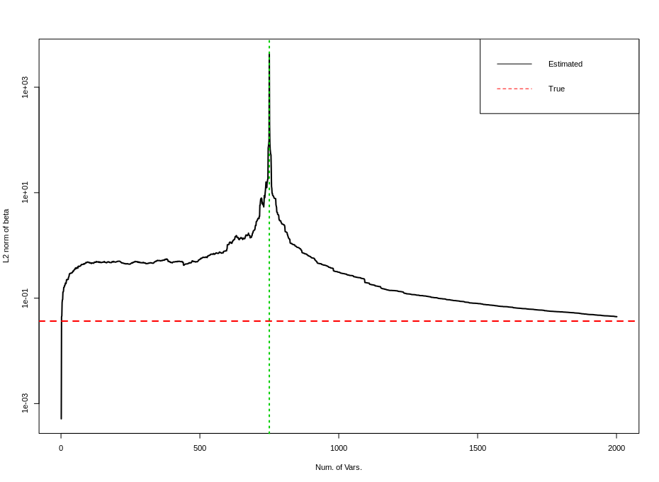
<p>代码只需要稍作修改即可, 结果如下.</p>

<p><img src="../assets/2021010815296.png" alt="image" style="zoom:46%;" />
<img src="../assets/2021010815297.png" alt="image" style="zoom:46%;" /></p>

<p>上面两张图分别是测试误差双下降曲线, 以及估计量的 \(\ell_2\) 范数随着变量增加的曲线. 
第一张图与上面其他所有图的最大不同点在于 bias 曲线在末尾持续下降到几乎为 0 (\(10^{-4}\) 量级), 此时测试误差曲线是影响测试误差的主要原因. 随着 \(p\) 增加该项会持续降低. (后文有讨论)</p>

<h3 id="32-summary-and-code">3.2 Summary and code</h3>

<div class="language-R highlighter-rouge"><div class="highlight"><pre class="highlight"><code><span class="n">set.seed</span><span class="p">(</span><span class="m">1111</span><span class="p">)</span><span class="w">
</span><span class="c1">## settings</span><span class="w">
</span><span class="n">n</span><span class="w"> </span><span class="o">&lt;-</span><span class="w"> </span><span class="m">1000</span><span class="w">
</span><span class="n">p</span><span class="w"> </span><span class="o">&lt;-</span><span class="w"> </span><span class="m">2000</span><span class="w">   </span><span class="c1"># 2000 2500</span><span class="w">
</span><span class="n">n_train</span><span class="w"> </span><span class="o">&lt;-</span><span class="w"> </span><span class="nf">as.integer</span><span class="p">(</span><span class="n">n</span><span class="w"> </span><span class="o">*</span><span class="w"> </span><span class="m">0.75</span><span class="p">)</span><span class="w">
</span><span class="n">n_test</span><span class="w"> </span><span class="o">&lt;-</span><span class="w"> </span><span class="n">n</span><span class="w"> </span><span class="o">-</span><span class="w"> </span><span class="n">n_train</span><span class="w">
</span><span class="c1">## model settings</span><span class="w">
</span><span class="n">mean_x</span><span class="w"> </span><span class="o">&lt;-</span><span class="w"> </span><span class="nf">c</span><span class="p">(</span><span class="nf">rep</span><span class="p">(</span><span class="m">0</span><span class="p">,</span><span class="n">p</span><span class="p">))</span><span class="w">
</span><span class="n">sigma_x</span><span class="w"> </span><span class="o">&lt;-</span><span class="w"> </span><span class="n">matrix</span><span class="p">(</span><span class="m">0</span><span class="p">,</span><span class="n">p</span><span class="p">,</span><span class="n">p</span><span class="p">)</span><span class="w">     
</span><span class="k">for</span><span class="w"> </span><span class="p">(</span><span class="n">i</span><span class="w"> </span><span class="k">in</span><span class="w"> </span><span class="m">1</span><span class="o">:</span><span class="n">p</span><span class="p">){</span><span class="w">
  </span><span class="k">for</span><span class="w"> </span><span class="p">(</span><span class="n">j</span><span class="w"> </span><span class="k">in</span><span class="w"> </span><span class="m">1</span><span class="o">:</span><span class="n">p</span><span class="p">){</span><span class="w">
    </span><span class="n">sigma_x</span><span class="p">[</span><span class="n">i</span><span class="p">,</span><span class="n">j</span><span class="p">]</span><span class="w"> </span><span class="o">&lt;-</span><span class="w"> </span><span class="m">0.90</span><span class="o">^</span><span class="nf">abs</span><span class="p">(</span><span class="n">i</span><span class="o">-</span><span class="n">j</span><span class="p">)</span><span class="w">
  </span><span class="p">}</span><span class="w">
</span><span class="p">}</span><span class="w">

</span><span class="n">mean_e</span><span class="w"> </span><span class="o">&lt;-</span><span class="w"> </span><span class="nf">c</span><span class="p">(</span><span class="nf">rep</span><span class="p">(</span><span class="m">0</span><span class="p">,</span><span class="n">n</span><span class="p">))</span><span class="w">
</span><span class="n">sigma_e</span><span class="w"> </span><span class="o">&lt;-</span><span class="w"> </span><span class="n">diag</span><span class="p">(</span><span class="n">x</span><span class="o">=</span><span class="m">1</span><span class="p">,</span><span class="n">n</span><span class="p">,</span><span class="n">n</span><span class="p">)</span><span class="w">
</span><span class="n">x</span><span class="w"> </span><span class="o">&lt;-</span><span class="w"> </span><span class="n">mvrnorm</span><span class="p">(</span><span class="n">n</span><span class="o">=</span><span class="n">n</span><span class="p">,</span><span class="n">mean_x</span><span class="p">,</span><span class="n">sigma_x</span><span class="p">)</span><span class="w">
</span><span class="n">x</span><span class="w"> </span><span class="o">&lt;-</span><span class="w"> </span><span class="n">x</span><span class="p">[,</span><span class="w"> </span><span class="n">sample</span><span class="p">(</span><span class="n">p</span><span class="p">)]</span><span class="w">                        </span><span class="c1"># disorder correlation</span><span class="w">
</span><span class="n">e</span><span class="w"> </span><span class="o">&lt;-</span><span class="w"> </span><span class="n">mvrnorm</span><span class="p">(</span><span class="n">n</span><span class="o">=</span><span class="m">1</span><span class="p">,</span><span class="n">mean_e</span><span class="p">,</span><span class="n">sigma_e</span><span class="p">)</span><span class="w"> </span><span class="o">*</span><span class="w"> </span><span class="m">2</span><span class="w">
</span><span class="n">beta0</span><span class="w"> </span><span class="o">&lt;-</span><span class="w"> </span><span class="nf">c</span><span class="p">(</span><span class="nf">rep</span><span class="p">(</span><span class="m">0</span><span class="p">,</span><span class="n">p</span><span class="p">))</span><span class="w">

</span><span class="c1">### setting beta0</span><span class="w">
</span><span class="c1">## default case</span><span class="w">
</span><span class="n">mean_beta</span><span class="w"> </span><span class="o">&lt;-</span><span class="w"> </span><span class="n">rbinom</span><span class="p">(</span><span class="m">2000</span><span class="p">,</span><span class="w"> </span><span class="m">10</span><span class="p">,</span><span class="w"> </span><span class="m">0.1</span><span class="p">)</span><span class="w"> </span><span class="o">*</span><span class="w"> </span><span class="m">4</span><span class="w">
</span><span class="n">beta0</span><span class="p">[</span><span class="m">1</span><span class="o">:</span><span class="m">2000</span><span class="p">]</span><span class="w"> </span><span class="o">&lt;-</span><span class="w"> </span><span class="n">mvrnorm</span><span class="p">(</span><span class="n">n</span><span class="o">=</span><span class="m">1</span><span class="p">,</span><span class="w"> </span><span class="n">mean_beta</span><span class="p">,</span><span class="w"> </span><span class="n">diag</span><span class="p">(</span><span class="m">2000</span><span class="p">))</span><span class="w">
</span><span class="n">beta0</span><span class="p">[(</span><span class="m">1</span><span class="o">:</span><span class="m">200</span><span class="p">)</span><span class="o">*</span><span class="m">2</span><span class="p">]</span><span class="w"> </span><span class="o">&lt;-</span><span class="w"> </span><span class="nf">rep</span><span class="p">(</span><span class="m">40</span><span class="p">,</span><span class="w"> </span><span class="m">200</span><span class="p">)</span><span class="w">
</span><span class="n">beta0</span><span class="p">[(</span><span class="m">801</span><span class="o">:</span><span class="m">1000</span><span class="p">)</span><span class="o">*</span><span class="m">2</span><span class="p">]</span><span class="w"> </span><span class="o">&lt;-</span><span class="w"> </span><span class="nf">rep</span><span class="p">(</span><span class="m">40</span><span class="p">,</span><span class="w"> </span><span class="m">200</span><span class="p">)</span><span class="w">
</span><span class="n">beta0</span><span class="p">[</span><span class="n">which</span><span class="p">(</span><span class="nf">abs</span><span class="p">(</span><span class="n">beta0</span><span class="p">)</span><span class="w"> </span><span class="o">&lt;</span><span class="w"> </span><span class="m">1e-1</span><span class="p">)]</span><span class="w"> </span><span class="o">&lt;-</span><span class="w"> </span><span class="m">0</span><span class="w">
</span><span class="n">beta0</span><span class="p">[</span><span class="m">500</span><span class="o">:</span><span class="m">1000</span><span class="p">]</span><span class="w"> </span><span class="o">&lt;-</span><span class="w"> </span><span class="m">0</span><span class="w">
</span><span class="c1">## zero bias curve case in Case 5</span><span class="w">
</span><span class="c1"># svd_x &lt;- svd(x, nv=p, nu=n_train)</span><span class="w">
</span><span class="c1"># beta0 &lt;- svd_x$$v[,1]</span><span class="w">
</span><span class="n">beta0</span><span class="w"> </span><span class="o">&lt;-</span><span class="w"> </span><span class="n">beta0</span><span class="w"> </span><span class="o">/</span><span class="w"> </span><span class="n">norm</span><span class="p">(</span><span class="n">beta0</span><span class="p">,</span><span class="n">type</span><span class="o">=</span><span class="s2">"2"</span><span class="p">)</span><span class="w"> </span><span class="o">*</span><span class="w"> </span><span class="m">8</span><span class="w">  </span><span class="c1"># control SNR</span><span class="w">
</span><span class="c1"># length(which(abs(beta0) &lt; 1e-3))         # for debug</span><span class="w">

</span><span class="c1"># linear model</span><span class="w">
</span><span class="n">y0</span><span class="w"> </span><span class="o">&lt;-</span><span class="w"> </span><span class="n">x</span><span class="w"> </span><span class="o">%*%</span><span class="w"> </span><span class="n">beta0</span><span class="w">
</span><span class="n">y</span><span class="w"> </span><span class="o">&lt;-</span><span class="w"> </span><span class="n">y0</span><span class="w"> </span><span class="o">+</span><span class="w"> </span><span class="n">e</span><span class="w">
</span><span class="c1">## some standardization</span><span class="w">
</span><span class="n">beta0</span><span class="w"> </span><span class="o">&lt;-</span><span class="w"> </span><span class="n">beta0</span><span class="w"> </span><span class="o">/</span><span class="w"> </span><span class="n">sd</span><span class="p">(</span><span class="n">y</span><span class="p">)</span><span class="w">
</span><span class="n">y0</span><span class="w"> </span><span class="o">&lt;-</span><span class="w"> </span><span class="n">y0</span><span class="w"> </span><span class="o">/</span><span class="w"> </span><span class="n">sd</span><span class="p">(</span><span class="n">y</span><span class="p">)</span><span class="w">
</span><span class="n">y</span><span class="w"> </span><span class="o">&lt;-</span><span class="w"> </span><span class="n">y</span><span class="w"> </span><span class="o">/</span><span class="w"> </span><span class="n">sd</span><span class="p">(</span><span class="n">y</span><span class="p">)</span><span class="w">
</span></code></pre></div></div>

<h2 id="4-code-for-calculation-paralleling-and-plotting">4. Code for calculation, paralleling and plotting</h2>

<h3 id="41-calculating-test-error">4.1 Calculating test error</h3>

<div class="language-R highlighter-rouge"><div class="highlight"><pre class="highlight"><code><span class="c1"># sample splitting</span><span class="w">
</span><span class="n">x</span><span class="w"> </span><span class="o">&lt;-</span><span class="w"> </span><span class="n">cbind</span><span class="p">(</span><span class="n">matrix</span><span class="p">(</span><span class="m">1</span><span class="p">,</span><span class="n">n</span><span class="p">,</span><span class="m">1</span><span class="p">),</span><span class="n">x</span><span class="p">)</span><span class="w">
</span><span class="n">x_train</span><span class="w"> </span><span class="o">&lt;-</span><span class="w"> </span><span class="n">x</span><span class="p">[</span><span class="m">1</span><span class="o">:</span><span class="n">n_train</span><span class="p">,]</span><span class="w">
</span><span class="n">x_test</span><span class="w"> </span><span class="o">&lt;-</span><span class="w"> </span><span class="n">x</span><span class="p">[(</span><span class="n">n_train</span><span class="m">+1</span><span class="p">)</span><span class="o">:</span><span class="n">n</span><span class="p">,]</span><span class="w">
</span><span class="n">y_train</span><span class="w"> </span><span class="o">&lt;-</span><span class="w"> </span><span class="n">y</span><span class="p">[</span><span class="m">1</span><span class="o">:</span><span class="n">n_train</span><span class="p">]</span><span class="w">
</span><span class="n">y_test</span><span class="w"> </span><span class="o">&lt;-</span><span class="w"> </span><span class="n">y</span><span class="p">[(</span><span class="n">n_train</span><span class="m">+1</span><span class="p">)</span><span class="o">:</span><span class="n">n</span><span class="p">]</span><span class="w">
</span><span class="n">y0_train</span><span class="w"> </span><span class="o">&lt;-</span><span class="w"> </span><span class="n">y0</span><span class="p">[</span><span class="m">1</span><span class="o">:</span><span class="n">n_train</span><span class="p">]</span><span class="w">
</span><span class="n">y0_test</span><span class="w"> </span><span class="o">&lt;-</span><span class="w"> </span><span class="n">y0</span><span class="p">[(</span><span class="n">n_train</span><span class="m">+1</span><span class="p">)</span><span class="o">:</span><span class="n">n</span><span class="p">]</span><span class="w">

</span><span class="c1"># oracle predict error</span><span class="w">
</span><span class="n">PE0</span><span class="w"> </span><span class="o">&lt;-</span><span class="w"> </span><span class="nf">as.numeric</span><span class="p">(</span><span class="n">t</span><span class="p">(</span><span class="n">y0_test</span><span class="w"> </span><span class="o">-</span><span class="w"> </span><span class="n">y_test</span><span class="p">)</span><span class="w"> </span><span class="o">%*%</span><span class="w"> </span><span class="p">(</span><span class="n">y0_test</span><span class="w"> </span><span class="o">-</span><span class="w"> </span><span class="n">y_test</span><span class="p">))</span><span class="w"> </span><span class="o">/</span><span class="w"> </span><span class="n">n_test</span><span class="w">
</span><span class="c1"># some criterias </span><span class="w">
</span><span class="n">norm_beta_hat</span><span class="w"> </span><span class="o">&lt;-</span><span class="w"> </span><span class="nf">rep</span><span class="p">(</span><span class="m">0</span><span class="p">,</span><span class="n">p</span><span class="m">+1</span><span class="p">)</span><span class="w">
</span><span class="n">test_error</span><span class="w"> </span><span class="o">&lt;-</span><span class="w"> </span><span class="nf">rep</span><span class="p">(</span><span class="m">0</span><span class="p">,</span><span class="n">p</span><span class="m">+1</span><span class="p">)</span><span class="w">
</span><span class="n">train_error</span><span class="w"> </span><span class="o">&lt;-</span><span class="w"> </span><span class="nf">rep</span><span class="p">(</span><span class="m">0</span><span class="p">,</span><span class="n">p</span><span class="m">+1</span><span class="p">)</span><span class="w">
</span><span class="n">bias</span><span class="w"> </span><span class="o">&lt;-</span><span class="w"> </span><span class="nf">rep</span><span class="p">(</span><span class="m">0</span><span class="p">,</span><span class="n">p</span><span class="m">+1</span><span class="p">)</span><span class="w">
</span><span class="n">variance</span><span class="w"> </span><span class="o">&lt;-</span><span class="w"> </span><span class="nf">rep</span><span class="p">(</span><span class="m">0</span><span class="p">,</span><span class="n">p</span><span class="m">+1</span><span class="p">)</span><span class="w">

</span><span class="c1"># main function</span><span class="w">
</span><span class="n">my_fun</span><span class="w"> </span><span class="o">&lt;-</span><span class="w"> </span><span class="k">function</span><span class="p">(</span><span class="n">num_featrues</span><span class="p">){</span><span class="w">
  </span><span class="n">x_train_tmp</span><span class="w"> </span><span class="o">&lt;-</span><span class="w"> </span><span class="n">as.matrix</span><span class="p">(</span><span class="n">x_train</span><span class="p">[,</span><span class="m">1</span><span class="o">:</span><span class="n">num_featrues</span><span class="p">])</span><span class="w">
  </span><span class="n">x_test_tmp</span><span class="w"> </span><span class="o">&lt;-</span><span class="w"> </span><span class="n">as.matrix</span><span class="p">(</span><span class="n">x_test</span><span class="p">[,</span><span class="m">1</span><span class="o">:</span><span class="n">num_featrues</span><span class="p">])</span><span class="w">
  </span><span class="k">if</span><span class="w"> </span><span class="p">(</span><span class="n">ncol</span><span class="p">(</span><span class="n">x_train_tmp</span><span class="p">)</span><span class="w"> </span><span class="o">&lt;=</span><span class="w"> </span><span class="n">nrow</span><span class="p">(</span><span class="n">x_train_tmp</span><span class="p">)){</span><span class="w">
    </span><span class="n">hat_matrix</span><span class="w"> </span><span class="o">&lt;-</span><span class="w"> </span><span class="n">solve</span><span class="p">(</span><span class="n">t</span><span class="p">(</span><span class="n">x_train_tmp</span><span class="p">)</span><span class="w"> </span><span class="o">%*%</span><span class="w"> </span><span class="n">x_train_tmp</span><span class="p">)</span><span class="w"> </span><span class="o">%*%</span><span class="w"> </span><span class="n">t</span><span class="p">(</span><span class="n">x_train_tmp</span><span class="p">)</span><span class="w">
    </span><span class="n">beta_hat</span><span class="w"> </span><span class="o">&lt;-</span><span class="w"> </span><span class="n">hat_matrix</span><span class="w"> </span><span class="o">%*%</span><span class="w"> </span><span class="n">y_train</span><span class="w">
    </span><span class="n">beta_hat_0</span><span class="w"> </span><span class="o">&lt;-</span><span class="w"> </span><span class="n">hat_matrix</span><span class="w"> </span><span class="o">%*%</span><span class="w"> </span><span class="n">y0_train</span><span class="w">
    </span><span class="c1"># beta_hat &lt;- decmps$$v %*% diag(1/decmps$$d) %*% t(decmps$$u[,1:length(decmps$$d)]) %*% y_train</span><span class="w">
  </span><span class="p">}</span><span class="w"> </span><span class="k">else</span><span class="w"> </span><span class="p">{</span><span class="w">
    </span><span class="n">decmps</span><span class="w"> </span><span class="o">&lt;-</span><span class="w"> </span><span class="n">svd</span><span class="p">(</span><span class="n">x_train_tmp</span><span class="p">,</span><span class="w"> </span><span class="n">nu</span><span class="o">=</span><span class="n">nrow</span><span class="p">(</span><span class="n">x_train_tmp</span><span class="p">),</span><span class="w"> </span><span class="n">nv</span><span class="o">=</span><span class="n">ncol</span><span class="p">(</span><span class="n">x_train_tmp</span><span class="p">))</span><span class="w">
    </span><span class="n">hat_matrix</span><span class="w"> </span><span class="o">&lt;-</span><span class="w"> </span><span class="n">decmps</span><span class="o">$$</span><span class="n">v</span><span class="w"> </span><span class="o">%*%</span><span class="w"> </span><span class="n">rbind</span><span class="p">(</span><span class="n">diag</span><span class="p">(</span><span class="m">1</span><span class="o">/</span><span class="n">decmps</span><span class="o">$$</span><span class="n">d</span><span class="p">),</span><span class="n">matrix</span><span class="p">(</span><span class="m">0</span><span class="p">,</span><span class="n">nrow</span><span class="o">=</span><span class="n">ncol</span><span class="p">(</span><span class="n">x_train_tmp</span><span class="p">)</span><span class="o">-</span><span class="n">nrow</span><span class="p">(</span><span class="n">x_train_tmp</span><span class="p">),</span><span class="n">ncol</span><span class="o">=</span><span class="n">nrow</span><span class="p">(</span><span class="n">x_train_tmp</span><span class="p">)))</span><span class="w"> </span><span class="o">%*%</span><span class="w"> </span><span class="n">t</span><span class="p">(</span><span class="n">decmps</span><span class="o">$$</span><span class="n">u</span><span class="p">[,</span><span class="m">1</span><span class="o">:</span><span class="nf">length</span><span class="p">(</span><span class="n">decmps</span><span class="o">$$</span><span class="n">d</span><span class="p">)])</span><span class="w">
    </span><span class="n">beta_hat</span><span class="w"> </span><span class="o">&lt;-</span><span class="w"> </span><span class="n">hat_matrix</span><span class="w"> </span><span class="o">%*%</span><span class="w"> </span><span class="n">y_train</span><span class="w">
    </span><span class="n">beta_hat_0</span><span class="w"> </span><span class="o">&lt;-</span><span class="w"> </span><span class="n">hat_matrix</span><span class="w"> </span><span class="o">%*%</span><span class="w"> </span><span class="n">y0_train</span><span class="w">
  </span><span class="p">}</span><span class="w">
  
  </span><span class="c1">## l2-norm of beta hat</span><span class="w">
  </span><span class="n">norm_beta_hat_cur</span><span class="w"> </span><span class="o">&lt;-</span><span class="w"> </span><span class="nf">as.numeric</span><span class="p">(</span><span class="n">t</span><span class="p">(</span><span class="n">beta_hat</span><span class="p">)</span><span class="w"> </span><span class="o">%*%</span><span class="w"> </span><span class="n">beta_hat</span><span class="p">)</span><span class="w">
  </span><span class="c1">## train error</span><span class="w">
  </span><span class="n">tmp_error</span><span class="w"> </span><span class="o">&lt;-</span><span class="w"> </span><span class="n">x_train_tmp</span><span class="w"> </span><span class="o">%*%</span><span class="w"> </span><span class="n">beta_hat</span><span class="w"> </span><span class="o">-</span><span class="w"> </span><span class="n">y_train</span><span class="w">
  </span><span class="n">train_error_cur</span><span class="w"> </span><span class="o">&lt;-</span><span class="w"> </span><span class="nf">as.numeric</span><span class="p">(</span><span class="n">t</span><span class="p">(</span><span class="n">tmp_error</span><span class="p">)</span><span class="w"> </span><span class="o">%*%</span><span class="w"> </span><span class="n">tmp_error</span><span class="p">)</span><span class="w">
  </span><span class="c1">## test error</span><span class="w">
  </span><span class="n">tmp_error</span><span class="w"> </span><span class="o">&lt;-</span><span class="w"> </span><span class="n">x_test_tmp</span><span class="w"> </span><span class="o">%*%</span><span class="w"> </span><span class="n">beta_hat</span><span class="w"> </span><span class="o">-</span><span class="w"> </span><span class="n">y_test</span><span class="w">
  </span><span class="n">test_error_cur</span><span class="w"> </span><span class="o">&lt;-</span><span class="w"> </span><span class="nf">as.numeric</span><span class="p">(</span><span class="n">t</span><span class="p">(</span><span class="n">tmp_error</span><span class="p">)</span><span class="w"> </span><span class="o">%*%</span><span class="w"> </span><span class="n">tmp_error</span><span class="p">)</span><span class="w">
  </span><span class="c1">## bias term</span><span class="w">
  </span><span class="c1"># tmp_error &lt;- x_test_tmp %*% beta_hat_0 - x_test[,-1] %*% beta0</span><span class="w">
  </span><span class="n">tmp_error</span><span class="w"> </span><span class="o">&lt;-</span><span class="w"> </span><span class="n">x_test_tmp</span><span class="w"> </span><span class="o">%*%</span><span class="w"> </span><span class="n">beta_hat_0</span><span class="w"> </span><span class="o">-</span><span class="w"> </span><span class="n">y0_test</span><span class="w">
  </span><span class="n">bias2</span><span class="w"> </span><span class="o">&lt;-</span><span class="w"> </span><span class="nf">as.numeric</span><span class="p">(</span><span class="n">t</span><span class="p">(</span><span class="n">tmp_error</span><span class="p">)</span><span class="w"> </span><span class="o">%*%</span><span class="w"> </span><span class="n">tmp_error</span><span class="p">)</span><span class="w">
  </span><span class="c1">## variance term</span><span class="w">
  </span><span class="n">tmp_error</span><span class="w"> </span><span class="o">&lt;-</span><span class="w"> </span><span class="n">x_test_tmp</span><span class="w"> </span><span class="o">%*%</span><span class="w"> </span><span class="p">(</span><span class="n">beta_hat_0</span><span class="w"> </span><span class="o">-</span><span class="w"> </span><span class="n">beta_hat</span><span class="p">)</span><span class="w">
  </span><span class="n">variance</span><span class="w"> </span><span class="o">&lt;-</span><span class="w"> </span><span class="nf">as.numeric</span><span class="p">(</span><span class="n">t</span><span class="p">(</span><span class="n">tmp_error</span><span class="p">)</span><span class="w"> </span><span class="o">%*%</span><span class="w"> </span><span class="n">tmp_error</span><span class="p">)</span><span class="w">
  
  </span><span class="c1"># outputs</span><span class="w">
  </span><span class="n">output</span><span class="w"> </span><span class="o">&lt;-</span><span class="w"> </span><span class="nf">c</span><span class="p">(</span><span class="n">train_error_cur</span><span class="p">,</span><span class="n">test_error_cur</span><span class="p">,</span><span class="n">norm_beta_hat_cur</span><span class="p">,</span><span class="n">bias2</span><span class="p">,</span><span class="n">variance</span><span class="p">)</span><span class="w">
  </span><span class="n">output</span><span class="w">
</span><span class="p">}</span><span class="w">

</span></code></pre></div></div>

<h3 id="42-paralleled-programming">4.2 Paralleled programming</h3>
<div class="language-R highlighter-rouge"><div class="highlight"><pre class="highlight"><code><span class="c1">## parallel</span><span class="w">
</span><span class="n">cl</span><span class="w"> </span><span class="o">&lt;-</span><span class="w"> </span><span class="n">makeCluster</span><span class="p">(</span><span class="n">detectCores</span><span class="p">()</span><span class="o">-</span><span class="w"> </span><span class="m">5</span><span class="p">)</span><span class="w">
</span><span class="n">clusterEvalQ</span><span class="p">(</span><span class="n">cl</span><span class="o">=</span><span class="n">cl</span><span class="p">,</span><span class="w"> </span><span class="n">library</span><span class="p">(</span><span class="n">MASS</span><span class="p">))</span><span class="w">
</span><span class="n">clusterExport</span><span class="p">(</span><span class="n">cl</span><span class="p">,</span><span class="w"> </span><span class="nf">c</span><span class="p">(</span><span class="s2">"x"</span><span class="p">,</span><span class="s2">"x_train"</span><span class="p">,</span><span class="s2">"x_test"</span><span class="p">,</span><span class="s2">"y_train"</span><span class="p">,</span><span class="s2">"y_test"</span><span class="p">,</span><span class="s2">"y0_train"</span><span class="p">,</span><span class="s2">"y0_test"</span><span class="p">,</span><span class="s2">"beta0"</span><span class="p">))</span><span class="w">
</span><span class="n">tt</span><span class="w"> </span><span class="o">&lt;-</span><span class="w"> </span><span class="n">parSapply</span><span class="p">(</span><span class="n">cl</span><span class="p">,</span><span class="w"> </span><span class="m">1</span><span class="o">:</span><span class="p">(</span><span class="n">p</span><span class="m">+1</span><span class="p">),</span><span class="w"> </span><span class="n">my_fun</span><span class="p">)</span><span class="w">
</span><span class="n">stopCluster</span><span class="p">(</span><span class="n">cl</span><span class="p">)</span><span class="w">

</span><span class="c1"># align resultsw</span><span class="w">
</span><span class="n">train_error</span><span class="w"> </span><span class="o">&lt;-</span><span class="w"> </span><span class="n">tt</span><span class="p">[</span><span class="m">1</span><span class="p">,]</span><span class="w"> </span><span class="o">/</span><span class="w"> </span><span class="n">n_train</span><span class="w">
</span><span class="n">test_error</span><span class="w"> </span><span class="o">&lt;-</span><span class="w"> </span><span class="n">tt</span><span class="p">[</span><span class="m">2</span><span class="p">,]</span><span class="w"> </span><span class="o">/</span><span class="w"> </span><span class="n">n_test</span><span class="w">
</span><span class="n">norm_beta_hat</span><span class="w"> </span><span class="o">&lt;-</span><span class="w"> </span><span class="n">tt</span><span class="p">[</span><span class="m">3</span><span class="p">,]</span><span class="w">
</span><span class="n">bias2</span><span class="w"> </span><span class="o">&lt;-</span><span class="w"> </span><span class="n">tt</span><span class="p">[</span><span class="m">4</span><span class="p">,]</span><span class="w"> </span><span class="o">/</span><span class="w"> </span><span class="n">n_test</span><span class="w">
</span><span class="n">variance</span><span class="w"> </span><span class="o">&lt;-</span><span class="w"> </span><span class="n">tt</span><span class="p">[</span><span class="m">5</span><span class="p">,]</span><span class="w"> </span><span class="o">/</span><span class="w"> </span><span class="n">n_test</span><span class="w">
</span></code></pre></div></div>

<h3 id="43-plot-the-resulting-curve">4.3 Plot the resulting curve</h3>
<div class="language-R highlighter-rouge"><div class="highlight"><pre class="highlight"><code><span class="c1">## plot the results</span><span class="w">
</span><span class="c1"># the double descent curve</span><span class="w">
</span><span class="n">t</span><span class="w"> </span><span class="o">&lt;-</span><span class="w"> </span><span class="m">1</span><span class="o">:</span><span class="p">(</span><span class="n">p</span><span class="m">+1</span><span class="p">)</span><span class="w">
</span><span class="n">plot</span><span class="p">(</span><span class="n">t</span><span class="p">,</span><span class="w"> </span><span class="n">test_error</span><span class="p">,</span><span class="w"> </span><span class="s2">"l"</span><span class="p">,</span><span class="w"> </span><span class="n">lty</span><span class="o">=</span><span class="m">1</span><span class="p">,</span><span class="w"> </span><span class="n">lwd</span><span class="o">=</span><span class="m">2</span><span class="p">,</span><span class="w"> </span><span class="n">col</span><span class="o">=</span><span class="m">1</span><span class="p">,</span><span class="w"> </span><span class="n">xlab</span><span class="o">=</span><span class="s2">"Num. of Vars."</span><span class="p">,</span><span class="w"> </span><span class="n">ylab</span><span class="o">=</span><span class="s2">"Test Error"</span><span class="p">,</span><span class="w"> </span><span class="n">main</span><span class="o">=</span><span class="s2">"Double Descent"</span><span class="p">,</span><span class="w"> </span><span class="n">ylim</span><span class="o">=</span><span class="nf">c</span><span class="p">(</span><span class="m">0.0001</span><span class="p">,</span><span class="nf">max</span><span class="p">(</span><span class="n">test_error</span><span class="p">)),</span><span class="w"> </span><span class="n">log</span><span class="o">=</span><span class="s2">"y"</span><span class="p">)</span><span class="w"> </span><span class="c1"># </span><span class="w">
</span><span class="n">abline</span><span class="p">(</span><span class="n">v</span><span class="o">=</span><span class="n">n_train</span><span class="p">,</span><span class="n">col</span><span class="o">=</span><span class="m">2</span><span class="p">,</span><span class="n">lwd</span><span class="o">=</span><span class="m">1</span><span class="p">,</span><span class="n">lty</span><span class="o">=</span><span class="m">2</span><span class="p">)</span><span class="w"> </span><span class="c1"># vertical line</span><span class="w">
</span><span class="n">abline</span><span class="p">(</span><span class="n">h</span><span class="o">=</span><span class="n">PE0</span><span class="p">,</span><span class="n">col</span><span class="o">=</span><span class="m">2</span><span class="p">,</span><span class="n">lwd</span><span class="o">=</span><span class="m">1</span><span class="p">,</span><span class="n">lty</span><span class="o">=</span><span class="m">3</span><span class="p">)</span><span class="w">     </span><span class="c1"># horizon line, oracle test error</span><span class="w">
</span><span class="n">lines</span><span class="p">(</span><span class="n">t</span><span class="p">,</span><span class="n">bias2</span><span class="p">,</span><span class="n">col</span><span class="o">=</span><span class="m">3</span><span class="p">,</span><span class="n">lwd</span><span class="o">=</span><span class="m">2</span><span class="p">,</span><span class="n">lty</span><span class="o">=</span><span class="m">3</span><span class="p">)</span><span class="w">
</span><span class="n">lines</span><span class="p">(</span><span class="n">t</span><span class="p">,</span><span class="n">variance</span><span class="p">,</span><span class="n">col</span><span class="o">=</span><span class="m">4</span><span class="p">,</span><span class="n">lwd</span><span class="o">=</span><span class="m">2</span><span class="p">,</span><span class="n">lty</span><span class="o">=</span><span class="m">3</span><span class="p">)</span><span class="w">
</span><span class="n">lines</span><span class="p">(</span><span class="n">t</span><span class="p">,</span><span class="w"> </span><span class="n">PE0</span><span class="o">+</span><span class="n">bias2</span><span class="o">+</span><span class="n">variance</span><span class="p">,</span><span class="w"> </span><span class="n">lty</span><span class="o">=</span><span class="m">2</span><span class="p">)</span><span class="w"> </span><span class="c1"># expected test error</span><span class="w">
</span><span class="n">op</span><span class="w"> </span><span class="o">&lt;-</span><span class="w"> </span><span class="n">par</span><span class="p">(</span><span class="n">cex</span><span class="w"> </span><span class="o">=</span><span class="w"> </span><span class="m">0.7</span><span class="p">)</span><span class="w">                </span><span class="c1"># scale the legend</span><span class="w">
</span><span class="n">legend</span><span class="p">(</span><span class="s2">"bottomleft"</span><span class="p">,</span><span class="n">legend</span><span class="o">=</span><span class="nf">c</span><span class="p">(</span><span class="s2">"Test error"</span><span class="p">,</span><span class="s2">"Interpolation"</span><span class="p">,</span><span class="s2">"Irreducible error"</span><span class="p">,</span><span class="s2">"Squared Bias"</span><span class="p">,</span><span class="s2">"Variance"</span><span class="p">),</span><span class="w"> </span><span class="n">col</span><span class="o">=</span><span class="nf">c</span><span class="p">(</span><span class="m">1</span><span class="p">,</span><span class="m">2</span><span class="p">,</span><span class="m">2</span><span class="p">,</span><span class="m">3</span><span class="p">,</span><span class="m">4</span><span class="p">),</span><span class="w"> </span><span class="n">lty</span><span class="o">=</span><span class="nf">c</span><span class="p">(</span><span class="m">1</span><span class="p">,</span><span class="m">2</span><span class="p">,</span><span class="m">3</span><span class="p">,</span><span class="m">3</span><span class="p">,</span><span class="m">3</span><span class="p">))</span><span class="w">

</span><span class="c1"># train error</span><span class="w">
</span><span class="n">plot</span><span class="p">(</span><span class="n">t</span><span class="p">,</span><span class="w"> </span><span class="n">train_error</span><span class="p">,</span><span class="w"> </span><span class="s2">"l"</span><span class="p">,</span><span class="w"> </span><span class="n">lty</span><span class="o">=</span><span class="m">1</span><span class="p">,</span><span class="w"> </span><span class="n">lwd</span><span class="o">=</span><span class="m">2</span><span class="p">,</span><span class="w"> </span><span class="n">col</span><span class="o">=</span><span class="m">1</span><span class="p">,</span><span class="w"> </span><span class="n">xlab</span><span class="o">=</span><span class="s2">"Num. of Vars."</span><span class="p">,</span><span class="w"> </span><span class="n">main</span><span class="o">=</span><span class="s2">"Train Error"</span><span class="p">)</span><span class="w">
</span><span class="n">abline</span><span class="p">(</span><span class="n">v</span><span class="o">=</span><span class="n">n_train</span><span class="p">,</span><span class="n">col</span><span class="o">=</span><span class="m">2</span><span class="p">,</span><span class="n">lwd</span><span class="o">=</span><span class="m">2</span><span class="p">,</span><span class="n">lty</span><span class="o">=</span><span class="m">2</span><span class="p">)</span><span class="w">

</span><span class="c1"># the U curve</span><span class="w">
</span><span class="n">plot</span><span class="p">(</span><span class="n">t</span><span class="p">,</span><span class="w"> </span><span class="n">test_error</span><span class="p">,</span><span class="w"> </span><span class="s2">"l"</span><span class="p">,</span><span class="w"> </span><span class="n">lty</span><span class="o">=</span><span class="m">1</span><span class="p">,</span><span class="w"> </span><span class="n">lwd</span><span class="o">=</span><span class="m">2</span><span class="p">,</span><span class="w"> </span><span class="n">col</span><span class="o">=</span><span class="m">1</span><span class="p">,</span><span class="w"> </span><span class="n">xlab</span><span class="o">=</span><span class="s2">"Num. of Vars."</span><span class="p">,</span><span class="w"> </span><span class="n">ylab</span><span class="o">=</span><span class="s2">"Test Error"</span><span class="p">,</span><span class="w"> </span><span class="n">main</span><span class="o">=</span><span class="s2">"U Curve"</span><span class="p">,</span><span class="w"> </span><span class="n">xlim</span><span class="o">=</span><span class="nf">c</span><span class="p">(</span><span class="m">0</span><span class="p">,</span><span class="n">n_train</span><span class="p">))</span><span class="w">

</span><span class="c1">## the curve of norm of beta_hat</span><span class="w">
</span><span class="n">plot</span><span class="p">(</span><span class="n">t</span><span class="p">,</span><span class="w"> </span><span class="n">norm_beta_hat</span><span class="p">,</span><span class="w"> </span><span class="s2">"l"</span><span class="p">,</span><span class="w"> </span><span class="n">lty</span><span class="o">=</span><span class="m">1</span><span class="p">,</span><span class="w"> </span><span class="n">lwd</span><span class="o">=</span><span class="m">2</span><span class="p">,</span><span class="w"> </span><span class="n">col</span><span class="o">=</span><span class="m">1</span><span class="p">,</span><span class="w"> </span><span class="n">xlab</span><span class="o">=</span><span class="s2">"Num. of Vars."</span><span class="p">,</span><span class="w"> </span><span class="n">ylab</span><span class="o">=</span><span class="s2">"L2 norm of beta"</span><span class="p">,</span><span class="w"> </span><span class="n">log</span><span class="o">=</span><span class="s2">"y"</span><span class="p">)</span><span class="w">
</span><span class="n">abline</span><span class="p">(</span><span class="n">h</span><span class="o">=</span><span class="nf">as.numeric</span><span class="p">(</span><span class="n">t</span><span class="p">(</span><span class="n">beta0</span><span class="p">)</span><span class="w"> </span><span class="o">%*%</span><span class="w"> </span><span class="n">beta0</span><span class="p">),</span><span class="n">col</span><span class="o">=</span><span class="m">2</span><span class="p">,</span><span class="n">lwd</span><span class="o">=</span><span class="m">2</span><span class="p">,</span><span class="n">lty</span><span class="o">=</span><span class="m">2</span><span class="p">)</span><span class="w">
</span><span class="n">abline</span><span class="p">(</span><span class="n">v</span><span class="o">=</span><span class="n">n_train</span><span class="p">,</span><span class="n">col</span><span class="o">=</span><span class="m">3</span><span class="p">,</span><span class="n">lwd</span><span class="o">=</span><span class="m">2</span><span class="p">,</span><span class="n">lty</span><span class="o">=</span><span class="m">3</span><span class="p">)</span><span class="w">
</span><span class="n">legend</span><span class="p">(</span><span class="s2">"topright"</span><span class="p">,</span><span class="w"> </span><span class="n">legend</span><span class="o">=</span><span class="nf">c</span><span class="p">(</span><span class="s2">"Estimated"</span><span class="p">,</span><span class="s2">"True"</span><span class="p">),</span><span class="w"> </span><span class="n">col</span><span class="o">=</span><span class="m">1</span><span class="o">:</span><span class="m">2</span><span class="p">,</span><span class="w"> </span><span class="n">lty</span><span class="o">=</span><span class="m">1</span><span class="o">:</span><span class="m">2</span><span class="p">)</span><span class="w">
</span></code></pre></div></div>]]></content><author><name>Huihang Liu</name></author><category term="statistics," /><category term="machine" /><category term="learning" /><summary type="html"><![CDATA[1. Model, estimation and simulation settings]]></summary></entry><entry><title type="html">Errors</title><link href="/errors/" rel="alternate" type="text/html" title="Errors" /><published>2020-12-25T00:00:00+00:00</published><updated>2020-12-25T00:00:00+00:00</updated><id>/errors</id><content type="html" xml:base="/errors/"><![CDATA[<h3 id="q--a">Q &amp; A</h3>

<ol>
  <li>
    <p>Why we estimate errors?</p>

    <blockquote>
      <p>We believe that when we perform regression or classification the smaller the error the better the model.</p>

      <p>So that we can select the best model from various, assess the performance of models, and also average models with weights, of course, in terms of errors. (Those are separate goals in statistics.)</p>
    </blockquote>
  </li>
  <li>
    <p>Why we should care about the conditional / expected test error?</p>

    <blockquote>
      <p>Conditional test error is the most natural thing to care about for a model we’ve fitted to a particular training set.</p>

      <p>Expected test error is a more fundamental characteristic of a learning algorithm, since it averages over the vagaries of whether you got lucky or not with your particular training set.</p>

      <p>In linear model, they are the same asymptotically.</p>
    </blockquote>
  </li>
  <li>
    <p>What’s the difference between those errors?</p>

    <blockquote>
      <p>As shown in the following.</p>
    </blockquote>
  </li>
  <li>
    <p>Is CV a good estimator of \(\operatorname{Err}_{\mathcal{T}}\) or \(\operatorname{Err}\)?</p>
  </li>
</ol>

<blockquote>
  <p>Examined by simulation in linear setting. (ESL, Section 7.12)</p>

  <ul>
    <li>10-fold CV does a better job than LOO CV in estimating \(\operatorname{Err}_{\mathcal{T}}\). (Counter-intuitive)</li>
    <li>10-fold CV does a better job than LOO CV in estimating \(\operatorname{Err}\). (Intuitive)</li>
  </ul>

  <p>It shows that the CV estimates expected test error better than it estimates conditional test error.</p>

  <p>Thus it is fortunate if we’re comparing machine learning algorithms, but unfortunate if we want to know how well the particular model we fit a particular training set.</p>

  <p>Intuitively, it makes sense to me that CV is not so great for conditional test error because the whole procedure is based on changing your training data. (For the the best estimate of conditional test error, you need a fixed separate test set. But it’s fair to ask why the tiny changes to the training set involved in LOO CV in particular suffice for this.)</p>
</blockquote>

<h3 id="setting-and-definition">Setting and Definition</h3>

<p>In the following, we assume that</p>

\[\begin{equation}
y = f(x) + \varepsilon, \text{ where } \mathrm{E}(\varepsilon) = 0
\end{equation}.\]

<p>Suppose we have a target variable \(y_{1}\) and a corresponding vector of inputs \(\mathbf{x}_{1}\) , and a prediction model \(\hat{f}(\mathbf{x}_1)\) that has been estimated from a training set \(\mathcal{T}=\{(y_i,\mathbf{x}_i)\}_{i=1}^n\).  Let \(\mathbf{y}=(y_1,\dots,y_n)^T\in\mathbb{R}^{n}\) and \(\mathbf{X}=(\mathbf{x_1}^T,\dots,\mathbf{x_n}^T)^T\in\mathbb{R}^{n\times p}\) be output and input of the training sample in the matrix form.</p>

<h4 id="1-loss">1. Loss</h4>

<p>Squared / absolute error loss of  \(\hat{f}(\mathbf{x}_1)\) corresponding to \(y_1\):</p>

\[\begin{equation}
\label{eq:loss}
L(y_1, \hat{f}(\mathbf{x}_1)) = \left\{\begin{array}{ll}
(y_1-\hat{f}(\mathbf{x}_1))^{2} &amp; \text { squared error } \\
|y_1-\hat{f}(\mathbf{x}_1)| &amp; \text { absolute error. }
\end{array}\right.
\end{equation}\]

<blockquote>
  <p>In likelihood framework, loss could be \(-2\times \text{log-likelihood}\).</p>
</blockquote>

<p>We focus on the squared error loss in the following.</p>

<h4 id="2-training-error">2. Training error</h4>

\[\begin{align}
\label{eq:training_error}
\overline{\mathrm{err}}
&amp; = \frac{1}{n} \sum_{i=1}^{n} L\left(y_{i}, \hat{f}\left(x_{i}\right)\right) \\
&amp; = \frac{1}{n} \sum_{i=1}^{n} \left(y_{i} - \hat{f}\left(x_{i}\right)\right)^2
\end{align}\]

<p>Training error is the average loss over the training sample.</p>

<h4 id="3-in-sample-error">3. In-sample error</h4>

<blockquote>
  <p>In-sample error (ESL,2008) is equal to the average prediction error in Shao(1997).</p>
</blockquote>

\[\begin{equation}
\label{eq:in-sample_error}
\mathrm{E}_{y}[n^{−1} \|\mathbf{y}_{new} − \hat{f} (\mathbf{X})\|_2^2 \mid \mathcal{T} ]
\end{equation}\]

<p>\(\mathbf{y}_{new}\) is a vector of \(n\) future (unknown) observations associated with \(\mathbf{X}\) and is independent of \(\mathbf{y}\) in \(\mathcal{T}\).</p>

<blockquote>
  <p>Remark: Minimizing \(L(f(\mathbf{x}), \hat{f}(\mathbf{x}))\) defined in \(\eqref{eq:loss}\) is equivalent to minimizing the in-sample error in \(\eqref{eq:in-sample_error}\). This is well known in linear model averaging/selection procedure. (Homoscedasticity).</p>

\[\begin{align}
&amp; \mathrm{E}[ n^{−1} \| \mathbf{y}_{new} − \hat{f} (\mathbf{X})\|_2^2 \mid \mathcal{T} ] \\
&amp; = \mathrm{E}[ n^{−1} \| f (\mathbf{X}) + \boldsymbol{\varepsilon}_{new} − \hat{f} (\mathbf{X})\|_2^2 \mid \mathcal{T} ] \notag\\
&amp; = \sigma_\epsilon^2 + L(f(\mathbf{X}), \hat{f}(\mathbf{X})). \notag
\end{align}\]
</blockquote>

<h4 id="4-test-error">4. Test error</h4>

<p>also known as generalization error or prediction error</p>

\[\begin{align}
\label{eq:test_error}
&amp; \operatorname{Err}_{\mathcal{T}} \\
&amp; = \mathrm{E}_{\mathbf{x}_{new},y_{new}} [(y_{new} - \hat{f} (\mathbf{x}_{new}))^2 \mid \mathcal{T}] \notag\\
&amp; = \mathrm{E}_{\mathbf{x}_{new},\varepsilon_{new}} [(f (\mathbf{x}_{new}) + \varepsilon_{new} - \hat{f} (\mathbf{x}_{new}))^2 \mid \mathcal{T}] \notag\\
&amp; = \sigma_\varepsilon^2 + \mathrm{E}_{\mathbf{x}_{new}} [(f (\mathbf{x}_{new}) - \hat{f} (\mathbf{x}_{new}))^2 \mid \mathcal{T}] \notag \\
&amp; = \sigma_\varepsilon^2 + \mathrm{E}_{\mathbf{x}_{new}} [(f (\mathbf{x}_{new}) - E_{\mathbf{x}_{new}}\hat{f} (\mathbf{x}_{new}) + E_{\mathbf{x}_{new}}\hat{f} (\mathbf{x}_{new}) - \hat{f} (\mathbf{x}_{new}))^2 \mid \mathcal{T}] \notag \\
&amp; = \sigma_\varepsilon^2 + \mathrm{E}_{\mathbf{x}_{new}} [(f (\mathbf{x}_{new}) - E_{\mathbf{x}_{new}}\hat{f} (\mathbf{x}_{new}))^2 \mid \mathcal{T}] + \mathrm{E}_{\mathbf{x}_{new}}[ ( E_{\mathbf{x}_{new}}\hat{f} (\mathbf{x}_{new}) - \hat{f} (\mathbf{x}_{new}))^2 \mid \mathcal{T}] \notag \\
&amp; =  \text {Irreducible Error} + \text {Bias}(\mathcal{T})^{2} + \text {Variance}(\mathcal{T}). \notag
\end{align}\]

<p>Note that the training set \(\mathcal{T}\) is fixed in expression \(\eqref{eq:test_error}\) and the point \((\mathbf{x}_{new},y_{new})\) is a new test data point, drawn from \(F\), the joint distribution of the data.</p>

<blockquote>
  <p>In fact, this is the expected risk of the learned model \(\hat{f}(\mathbf{x})\) given the training set.</p>
</blockquote>

<p>The test error measures the predicted performance of the learned model on unknown data, that is, the generalization ability. If the generalization error of one learning method (algorithm) is lower than that of another method, then we believe that the former is more effective.</p>

<p>Remark: The generalization ability is related to the choice of the training set. If the number of samples in the training set are too small or under-represented, the generalization ability will be correspondingly weakened, meanwhile, the test error will increase.</p>

<h4 id="5-expected-test-error">5. Expected test error</h4>
<p>It is also known as expected prediction error which average the test error \(\operatorname{Err}_{\mathcal{T}}\) over training sets \(\mathcal{T}\) yields the expected error.</p>

<p>If we control the input value \(\mathbf{x}\) and just let \(y\), say \(\varepsilon\) be random. Then the (so called) “expected test error” of a regression fit \(\hat{f}(\mathbf{x})\) at an input point \(\mathbf{x} = \mathbf{x}_0\) can be decomposed as following</p>

\[\begin{align}
\label{eq:expected_test_error}
\operatorname{Err}(\mathbf{x}_{0}) 
&amp; = \mathrm{E}_{\varepsilon}\left[\left(y-\hat{f}(\mathbf{x})\right)^{2} \mid \mathbf{x}=\mathbf{x}_{0}\right] \\
&amp; = \sigma_{\varepsilon}^{2} + \left[\mathrm{E} \hat{f}(\mathbf{x}_{0}) - f(\mathbf{x}_{0})\right]^{2} + E\left[\hat{f}(\mathbf{x}_{0})-\mathrm{E} \hat{f}(\mathbf{x}_{0})\right]^{2} \notag\\
&amp; = \sigma_{\varepsilon}^{2} + \operatorname{Bias}^{2}\left(\hat{f}(\mathbf{x}_{0})\right) + \operatorname{Var}\left(\hat{f}(x_{0})\right) \notag\\
&amp; = \text { Irreducible Error }+\text { Bias }^{2} + \text { Variance. } \notag
\end{align}\]

<p>In linear model, we have</p>

\[=\quad \sigma_{\varepsilon}^{2}+\left[f\left(x_{0}\right)-\mathrm{E} \hat{f}_{p}\left(x_{0}\right)\right]^{2}+\left\|\mathbf{h}\left(x_{0}\right)\right\|^{2} \sigma_{\varepsilon}^{2}\]

<p>It measures the quality of the prediction method itself, that is, under any given training set, the average prediction ability that the prediction method can get. It measures not the generalization ability, but the prediction ability of the method itself with a fixed number of samples in training set.</p>

<h3 id="training-or-test-error">Training or Test Error</h3>

<p><img src="..\assets\image-20201226212751345.png?lastModify=1609045463" alt="image-20201226212751345" style="zoom:50%;" /></p>

<p>In the Figure, Lasso is used to produce the fits. Model complexity is the number of variables used (in linear settings).</p>

<ul>
  <li>Training error is not a good estimate of the test error, as seen in Figure above.</li>
</ul>

<p>There is some intermediate model complexity that gives minimum expected test error. Training error consistently decreases with model complexity, typically dropping to zero if we increase the model complexity enough. However, a model with zero training error is overfit to the training data and will typically generalize poorly.</p>

<h3 id="conditional-or-expected-test-error">Conditional or Expected Test Error</h3>

<p>Test error \(\operatorname{Err}_{\mathcal{T}}\) in \(\eqref{eq:test_error}\) is the error conditional on a given training set \(\mathcal{T}\), as opposed to the expected test error \(\operatorname{Err}\) in \(\eqref{eq:expected_test_error}\) which is an average over all sorts of training sets (we’re may never going to get to use).</p>

<p>\(\mathrm{Err}\) is more amenable to statistical analysis than the conditional one, and most methods effectively estimate the expected error. It does not seem possible to estimate conditional error effectively, given only the information in the same training set.</p>

<h5 id="simulation">Simulation</h5>

<p>Model setting: linear model with \(10\) true variables.</p>

<p><img src="..\assets\image-20201227111815932.png" alt="image-20201227111815932" style="zoom:50%;" /></p>

<p><strong>Figure</strong>. The thick red curve is the expected prediction error \(\mathrm{Err}\) . While, the thick black curves are the expected CV curves \(\mathrm{E}_{\mathcal{T}}\mathrm{CV}_{10}\) and \(\mathrm{E}_{\mathcal{T}}\mathrm{CV}_{n}\) . The lower-right panel shows the mean absolute deviation of the CV curves from the conditional error, \(\mathrm{E}_{\mathcal{T}}\vert\mathrm{CV}_{K}-\mathrm{Err}_{\mathcal{T}}\vert\) , as well as from the expected error \(\mathrm{E}_{\mathcal{T}}\vert\mathrm{CV}_{K}-\mathrm{Err}\vert\) for \(K={10,n}\).</p>

<p>It shows that both 10-fold CV and LOO CV are approximately unbiased for \(\operatorname{Err}\). 10-fold CV performs better than LOO CV.</p>

<p>We conclude that estimation of test error for a particular training set is not easy in general, given just the data from that same training set. Instead, cross-validation and related methods may provide reasonable estimates of the expected error \(\mathrm{Err}\).</p>

<p>This example tells us that in practice, for a given training set, it is difficult for us to estimate the generalization error.</p>

<h4 id="泛化误差上界">泛化误差上界</h4>

<p>统计学习方法 (李航, 第二版, Section 1.6.2) 给出了二分类问题的泛化误差的上界定理.</p>

<p><img src="../assets/image-20201227131616356.png" alt="image-20201227131616356" /></p>

<p>(1.32) 中, 左边是泛化误差, 右边为其上界, 其中 \(\hat{R}(f)\) 为训练误差; \(\varepsilon\) 是一个很小的量, 它随着样本大小 N 递减.</p>

<p>这个定理的条件较严格, 它要求函数空间是有限个函数组成的, 而且训练样本从总体中随机抽样. 李航说, 在一般的条件下, 该定理不容易得到.</p>]]></content><author><name>Huihang Liu</name></author><category term="statistics," /><category term="machine" /><category term="learning" /><summary type="html"><![CDATA[Q &amp; A]]></summary></entry><entry><title type="html">Double machine learning</title><link href="/dml/" rel="alternate" type="text/html" title="Double machine learning" /><published>2018-07-22T04:00:00+00:00</published><updated>2018-07-22T04:00:00+00:00</updated><id>/dml</id><content type="html" xml:base="/dml/"><![CDATA[<p>Source Ref: <a href="http://jmarkhou.com/dml/">jmarkhou’s Blog</a></p>

<p><a href="https://arxiv.org/abs/1608.00060">Interesting paper</a> by some fairly serious MIT-related econometrics/statistics people (let’s call this paper DML) on how to estimate some low-dimensional parameters of interest in the presence of high-dimensional nuisance parameters.  The intuition is quite nice, though the actual theoretical results are maybe not as generally applicable as they might appear at first.</p>

<h3 id="i-setup-and-results">I. Setup and results</h3>
<ul>
  <li>we want to estimate some finite-dimensional parameter $\theta$</li>
  <li>there is some very complicated nuisance parameter $\eta$ that we don’t care about
    <ul>
      <li>we’ll want to use fancy machine learning stuff to deal with $\eta$</li>
    </ul>
  </li>
  <li>the true value of $\theta$ and $\eta$ are $\theta_0$ and $\eta_0$</li>
  <li>we have some score function $\phi$ that is zero only at the true parameter values:
\(\begin{equation}
\mathbb{E}[\phi(W, \theta_0, \eta_0)] = 0
\tag{1}
\label{momentcondition}
\end{equation}\)
where data $W$ is generated IID from some distribution $\mathbb{P}$, and $\mathbb{E}$ denote the expectation wrt $\mathbb{P}$</li>
  <li>for a concrete example, think about the case of a simple linear regression:
    <ul>
      <li>$\phi$ would be the derivative of the least squares objective</li>
      <li>$\theta$ and $\eta$ would be the coefficients</li>
      <li>$\eqref{momentcondition}$ would be the first order conditions, which hold only at the true parameter values</li>
    </ul>
  </li>
</ul>

<p>DML recommends this procedure:</p>
<ol>
  <li>use a score $\phi$ that satisfies a <strong>Neyman orthogonality</strong> condition:
    <ul>
      <li>the directional derivative $\partial_{\eta}\mathbb{E}[\phi(W,\theta_0,\eta_0)][\eta-\eta_0] = 0$ for every $\eta$</li>
      <li>where $\partial_{\eta}f(x_0)[x-x_0] := \partial_t f(x_0+t(x-x_0)) $ is the directional derivative</li>
      <li>often, you can transform your $\phi$ so that it satisfies Neyman orthogonality</li>
    </ul>
  </li>
  <li>do <strong>cross-fitting</strong>, where you split your data into a main sample and an auxiliary sample, and:
    <ul>
      <li>use the auxiliary sample to train some fancy machine learning model to predict the nuisance parameter $\eta$</li>
      <li>on the main sample:
        <ul>
          <li>use this trained model to get $\hat{\eta}$</li>
          <li>then plug this into the empirical analogue of $\eqref{momentcondition}$ and solve for $\theta$, so that
  \(\mathbb{E}_n[\phi(W, \hat{\theta}, \hat{\eta})] = 0\)
   implicitly defines $\hat{\theta}$ (where $\mathbb{E}_n$ here denotes averaging over the main sample)</li>
        </ul>
      </li>
    </ul>
  </li>
  <li>this $\hat{\theta}$ will then be $\sqrt{n}$-consistent for $\theta_0$</li>
</ol>

<p>These two things (Neyman orthogonality and cross-fitting) are what gives us $\sqrt{n}$-consistency:</p>
<ul>
  <li>Neyman orthogonality makes $\phi$ insensitive to the nuisance parameter $\eta$ near the truth, so that plugging in an estimate of $\eta$ won’t hurt too much.</li>
  <li>Cross-fitting (as opposed to using the same data for both steps above) gives us a better estimate of $\hat{\eta}$, since the main sample where we plug $\hat{\eta}$ in to $\phi$ and then estimate $\hat{\theta}$ isn’t use when training the fancy ML model for predicting $\phi$ and thus $\hat{\eta}$ on the sample shouldn’t suffer from much overfitting.</li>
</ul>

<p>We’ll give a slightly deeper intuitive understanding for where these two conditions come from, as well as some considerations on how applicable this might be in practice.</p>

<h3 id="ii-intuition">II. Intuition</h3>

<h4 id="ii1-first-without-the-nuisance-parameter">II.1. First, without the nuisance parameter:</h4>
<p>If we knew the true value of the nuisance parameter $\eta_0$, we could just plug it into the empirical analogue of $\eqref{momentcondition}$ and solve for $\theta$ to get an estimate $\hat{\theta}_n$:</p>

<p>$ \mathbb{E}_n[\phi(X, \hat{\theta}_n, \eta_0)] = 0 $</p>

<p>For sufficiently large $n$, $\hat{\theta}_n$ will be pretty close to $\theta_0$ and $\phi$ will be approximately linear, so we can get the asymptotic distribution of $\hat{\theta}$:</p>

\[\begin{align}
0 &amp;= \mathbb{E}_n\phi(X, \hat{\theta}_n, \eta_0) 
\approx \mathbb{E}_n\phi(X, \theta_0, \eta_0) + \partial_{\theta}\mathbb{E}_n[\phi(W, \theta_0, \eta_0)](\hat{\theta}_n-\theta_0) \newline
&amp;\Rightarrow \partial_{\theta}\mathbb{E}_n[\phi(W, \theta_0, \eta_0)] \sqrt{n} (\hat{\theta}_n-\theta_0) \approx - \sqrt{n}\mathbb{E}_n\phi(X, \theta_0, \eta_0) \newline
&amp;\Rightarrow \sqrt{n} (\hat{\theta}_n-\theta_0) \rightarrow_d N(0, J^{-1}\Omega J^{-1\prime})
\tag{2}
\label{expansion0}
\end{align}\]

<p>where $J:= \partial_{\theta}\mathbb{E}[\phi(W, \theta_0, \eta_0)]$ and $\Omega := \mathrm{Var}\left[\phi(W, \theta_0, \eta_0)\right]$.</p>

<p>That is, assuming we know the true nuisance parameter $\eta_0$, our estimator $\hat{\theta}_n$ is $\sqrt{n}$-consistent, which is pretty nice.</p>

<h4 id="ii2-now-with-the-nuisance-parameter">II.2. Now, with the nuisance parameter:</h4>
<p>Unfortunately:</p>
<ul>
  <li>we don’t know $\eta_0$</li>
  <li>we still need to estimate $\theta_0$</li>
  <li>we’d still like to get this same $\sqrt{n}$-consistency</li>
</ul>

<p>To estimate $\theta_0$ in this case, probably the most natural thing to do is:</p>
<ol>
  <li>get a preliminary estimate for $\hat{\eta}_n$ of $\eta$</li>
  <li>pretend $\hat{\eta}_n \approx \eta_0$, and then do the same thing we did before where we solve for $\hat{\theta}_n$ using the empirical analogue of $\eqref{momentcondition}$:
\(\begin{equation}
\mathbb{E}_n[\phi(X, \hat{\theta}_n, \hat{\eta}_n)] = 0 
\tag{3}
\label{empiricalmomentcondition}
\end{equation}\)</li>
</ol>

<p>Note that so long as this nuisance parameter estimate $\hat{\eta}_n$ converges to the truth and $\phi$ is smooth, the argmax wrt $\theta$ of $\mathbb{E}_n[\phi]$ should also be smooth, so we should still get $\hat{\theta}\rightarrow\theta_0$.  So we can expand $\eqref{empiricalmomentcondition}$ around $\theta_0$:</p>

\[\begin{align}
0 &amp;= \mathbb{E}_n[\phi(X, \hat{\theta}_n, \hat{\eta}_n)] \approx \mathbb{E}_n[\phi(X, \theta_0, \hat{\eta}_n)] 
		+  \partial_{\theta}\mathbb{E}_n[\phi(X, \theta_0, \hat{\eta}_n)] (\hat{\theta}_n-\theta_0) \newline
&amp;\Rightarrow \partial_{\theta}\mathbb{E}_n[\phi(X, \theta_0, \hat{\eta}_n)] (\hat{\theta}_n-\theta_0) \sqrt{n}
		\approx - \sqrt{n} \mathbb{E}_n[\phi(X, \theta_0, \hat{\eta}_n)]  
\tag{4}
\label{expansion1}
\end{align}\]

<p>Basically, this looks a lot like $\eqref{expansion0}$, except with some $\hat{\eta}_n$s instead of $\eta_0$.  If we could make this look exactly like $\eqref{expansion0}$ as $n$ gets big, then we would get $\sqrt{n}$-consistency of $\hat{\theta}_n$ even in this case where we don’t know the true $\eta_0$ and have to plug in $\hat{\eta}_n$.</p>
<ul>
  <li>the left hand side is easy:
    <ul>
      <li>$\partial_{\theta}\mathbb{E}_n[\phi(X, \theta_0, \hat{\eta}_n)] $ is just an average</li>
      <li>so it should easily go to $J$ as $n$ gets big so long as $\phi$ is smooth and $\hat{\eta}_n$ converges to $\eta$</li>
      <li>so the left side of $\eqref{expansion1}$ will look like the left side of $\eqref{expansion0}$ as $n$ gets big</li>
    </ul>
  </li>
  <li>the right hand side $\sqrt{n} \mathbb{E}_n[\phi(X, \theta_0, \hat{\eta}_n)]$ is more involved:
    <ul>
      <li>in order to make this resemble the right side of $\eqref{expansion0}$, we need 
  \(\sqrt{n} \mathbb{E}_n[\phi(X, \theta_0, \hat{\eta}_n)] - \sqrt{n} \mathbb{E}_n[\phi(X, \theta_0, \hat{\eta}_0)] \rightarrow_p 0\)</li>
      <li>can use a stochastic equicontinuity argument if we’re using non-ML methods to get $\hat{\eta}_n$ (see Andrews 1994)</li>
      <li>but that argument minimally requires the set of potential $\hat{\eta}_n$ have finite VC dimension, whereas in modern ML applications typically we’ll fit increasingly complex functions as sample size increases, so this kind of classical argument doesn’t work</li>
    </ul>
  </li>
</ul>

<p>So instead, let’s continue with $\eqref{expansion1}$ and expand the RHS:</p>

<p>\(\begin{align}
&amp; \partial_{\theta}\mathbb{E}_n[\phi(X, \theta_0, \hat{\eta}_n)] (\hat{\theta}_n-\theta_0) \sqrt{n} \newline
&amp;\approx - \sqrt{n} \mathbb{E}_n[\phi(X, \theta_0, \hat{\eta}_n)]  \newline
&amp;\approx - \sqrt{n} 
			\mathbb{E}_n
			\left[
			\phi(X, \theta_0, \eta_0)
			+ \partial_{\eta}\phi(X, \theta_0, \eta_0)[\hat{\eta}_n-\eta_0]
			+ \frac{1}{2}\partial_{\eta^2}\phi(X, \theta_0, \eta_0)[\hat{\eta}_n-\eta_0]
			\right]
\tag{5}
\label{expansion2}
\end{align}\)
where :</p>
<ul>
  <li>$\partial_{\eta}\phi(X, \theta_0, \eta_0)[\hat{\eta}_n-\eta_0]$ is the directional derivative of $\phi$ wrt $\eta$ in the direction of $[\hat{\eta}-\eta_0]$</li>
  <li>$\partial_{\eta^2}\phi(X, \theta_0, \eta_0)[\hat{\eta}_n-\eta_0]$ the second derivative in that direction</li>
  <li>we’ve included the second derivative here since it’s not ex-ante obvious that it’ll vanish</li>
</ul>

<p>In order to make $\eqref{expansion2}$ look like $\eqref{expansion0}$ (and thus get $\sqrt{n}$-consistency for $\hat{\theta}_n$ ), we just need \(\sqrt{n} \mathbb{E}_n[\partial_{\eta} \phi (X, \theta_0, \eta_0) [\hat{\eta}_n - \eta_0]]\) and \(\sqrt{n} \mathbb{E}_n [\partial_{\eta^2}\phi(X, \theta_0, \eta_0)[\hat{\eta}_n-\eta_0]]\) to both go to 0.  Here’s where Neyman orthogonality and cross-fitting come in:</p>

<ol>
  <li>the Neyman (near)-orthogonality condition pretty much just amounts to assuming that \(\sqrt{n} \mathbb{E}_n[\partial_{\eta}\phi(X, \theta_0, \eta_0)[\hat{\eta}_n-\eta_0]]\) goes to 0</li>
  <li>Cross-fitting + assumption that $|\hat{\eta}-\eta_0|_2 = o_p(n^{-1/4})$ on hold-out data gives us \(\sqrt{n} \mathbb{E}_n[\partial_{\eta^2}\phi(X, \theta_0, \eta_0)[\hat{\eta}-\eta_0]]\) going to 0
    <ul>
      <li>the $| \hat{\eta}_n-\eta_0|_2 = o_p(n^{-1/4})$ guarantees that \(\mathbb{E}_n[\partial_{\eta^2}\phi(X, \theta_0, \eta_0)[\hat{\eta}_n-\eta_0]]\) will be $o_p(n^{-1/2})$
        <ul>
          <li>to see this, just consider the case where $\eta$ is 1-dimensional, where this second directional derivative is just $\partial_{\eta^2}\phi(X, \theta_0, \eta_0) (\hat{\eta}_n-\eta_0)^2$</li>
          <li>basically the same thing in general so long as $\phi$ is smooth</li>
        </ul>
      </li>
      <li>the cross-fitting just means that we estimate $\hat{\eta}_n$ on an auxiliary sample that we then don’t re-use when estimating $\theta$, so that we get the $o(n^{-1/4})$ rate for $\hat{\eta}_n$ when where we’re plugging in $\hat{\eta}_n$ and using it to estimate $\theta$ the main sample</li>
    </ul>
  </li>
</ol>

<p>A bit more intuition:</p>
<ul>
  <li>that we need a Neyman orthogonality condition seems reasonable:
    <ul>
      <li>we’re plugging in an estimate of the nuisance parameter $\eta$ to stand in for the truth $\eta_0$ when we estimate $\theta$</li>
      <li>so if the equation we solve to estimate $\theta$ depends on the value of this nuisance parameter then small errors in the nuisance parameter will mess things up</li>
      <li>Neyman orthogonality just says that this dependence gets small as our data gets big</li>
    </ul>
  </li>
  <li>estimating $\eta$ on an auxiliary data set separate from the data we use to estimate $\theta$ is basically to just control for overfitting
    <ul>
      <li>if we used the same data for estimating the $\eta$ as $\theta$, then the expectations in $\eqref{expansion2}$ would all be relative to the data that $\eta$ was estimated on</li>
      <li>as a result, these in-sample estimates of $\eta$ could overfit, and thus might not converge to $\eta_0$ at the required rate</li>
      <li>as an aside:  if we don’t do cross-fitting, but rather find other ways to limit in-sample overfitting, then everything should still be fine
        <ul>
          <li>the DML authors have some other work where they take this approach</li>
        </ul>
      </li>
    </ul>
  </li>
</ul>

<h3 id="iii-caveats">III. Caveats</h3>

<h4 id="iii1-the-set-of-ml-algorithms-dml-theory-applies-to">III.1. The set of ML algorithms DML theory applies to</h4>
<p>In general, $\sqrt{n}$-consistency of $\hat{\theta}_n$ requires that $|\hat{\eta}-\eta_0|_2 = o_p(n^{-1/4})$.  That is, whatever machine learning algorithm you’re using to approximate $\eta$ has to exhibit $L_2$ convergence at this rate.  Even in the special case where the second derivative \(\mathbb{E}[\partial_{\eta^2}\phi(X, \theta_0, \eta_0)[\eta-\eta_0]]\) is 0 for all $\eta$, you still need $L_2$ convergence.  The DML paper lists several examples of algorithms / problem settings with existing theoretical results that give this rate, but none of them are really <em>that</em> close to things you might do in practice:</p>
<ul>
  <li>Lasso for sparse models: this applies when the nuisance parameter is some linear function of a sparse set of parameters, which is a bit of an implausible assumption most of the time.</li>
  <li>Neural networks: the Chen White neural network result is for shallow feedforward networks.</li>
  <li>Boosting: the Luo Spindler result assumes the truth is a sparse linear model, and the base learning in the boosting algorithm here are univariate linear regressions, which is quite different from the popular tree boosting stuff that people often do in practice</li>
  <li>Trees/forests: the Wager Walther concentration result applies to convergence of a trained tree to the best theoretical tree with the same splits, and doesn’t say anything about approximating some true conditional mean.</li>
</ul>

<p>Also, I assume the Wager Athey random forest result is not mentioned because that convergence result is pointwise rather than $L_2$.</p>

<p>So, DML doesn’t actually provide much in the way of theoretical guarantees for estimating the nuisance parameter $\eta$ via ML methods that provide actually competitive predictive performance, e.g. tree boosting / random forests / deeper neural networks, since the necessary convergence results don’t yet exist for these methods.</p>

<h4 id="iii2-the-neyman-orthogonalization-procedure">III.2. The Neyman orthogonalization procedure</h4>
<p>The DML procedure requires that we have some score $\phi$ that satisfies Neyman orthogonality.  This is generically not the case, so we would like to have some way of transforming an arbitrary $\phi$ into something that satisfies Neyman orthogonality.  The DML paper provides illustrations of how to do this for a variety of different cases, and applies them to specific leading examples that economists find interesting.  However, it’s not entirely clear how generalizable these procedures are, especially when $\eta$ is a complicated thing we’re approximating by general ML methods.</p>

<p>For example, the ‘concentrating-out’ approach for Neyman orthogonalization in the case of M-estimation with infinite-dimensional nuisance parameters (section 2.23 in the DML paper) requires computing the optimal nuisance parameter $\eta$ as a function of the parameter of interest $\theta$, and then computing the derivative wrt $\theta$ of this function-valued mapping from $\theta$ to optimal $\eta$.  This approach is then applied to the leading example of interest (partially linear models with nuisance parameter) where the mapping from $\theta$ to optimal $\eta$ is fairly easy to compute and differentiate, due to the particular functional forms involved.  It seems like in most cases that are less straightforward, it’s not going to be so easy / possible to do this.</p>

<p>The DML paper presents a variety of other ways to orthogonalize stuff, and works out some more economics-relevant examples.  However, in general cases with high-dimensional nuisance parameters, it doesn’t appear that there’s a mechanical way to orthogonalize the score.  As a result, it may be necessary to manually orthogonalize before the DML procedure can be applied.</p>

<h3 id="references">References</h3>
<ul>
  <li><a href="https://arxiv.org/abs/1608.00060">Double/Debiased Machine Learning for Treatment and Causal Parameters</a></li>
  <li><a href="http://dido.econ.yale.edu/~dwka/pub/p0863.pdf">Andrews 1994 Asymptotics for Semiparametric Econometric Models via Stochastic Equicontinuity</a></li>
  <li><a href="https://arxiv.org/abs/1602.08927">Luo Spindler linear boosting convergence rate</a></li>
  <li><a href="https://arxiv.org/abs/1503.06388">Wager Walther tree concentration rate</a></li>
  <li><a href="https://ieeexplore.ieee.org/document/749011/">Chen White neural network convergence rate</a></li>
  <li><a href="https://arxiv.org/abs/1510.04342">Wager Athey pointwise asymptotic normality of random forests</a></li>
</ul>]]></content><author><name>jmarkhou</name></author><category term="statistics," /><category term="machine" /><category term="learning" /><summary type="html"><![CDATA[Source Ref: jmarkhou’s Blog]]></summary></entry></feed>