Errors
Q & A
-
Why we estimate errors?
We believe that when we perform regression or classification the smaller the error the better the model.
So that we can select the best model from various, assess the performance of models, and also average models with weights, of course, in terms of errors. (Those are separate goals in statistics.)
-
Why we should care about the conditional / expected test error?
Conditional test error is the most natural thing to care about for a model we’ve fitted to a particular training set.
Expected test error is a more fundamental characteristic of a learning algorithm, since it averages over the vagaries of whether you got lucky or not with your particular training set.
In linear model, they are the same asymptotically.
-
What’s the difference between those errors?
As shown in the following.
-
Is CV a good estimator of \(\operatorname{Err}_{\mathcal{T}}\) or \(\operatorname{Err}\)?
Examined by simulation in linear setting. (ESL, Section 7.12)
- 10-fold CV does a better job than LOO CV in estimating \(\operatorname{Err}_{\mathcal{T}}\). (Counter-intuitive)
- 10-fold CV does a better job than LOO CV in estimating \(\operatorname{Err}\). (Intuitive)
It shows that the CV estimates expected test error better than it estimates conditional test error.
Thus it is fortunate if we’re comparing machine learning algorithms, but unfortunate if we want to know how well the particular model we fit a particular training set.
Intuitively, it makes sense to me that CV is not so great for conditional test error because the whole procedure is based on changing your training data. (For the the best estimate of conditional test error, you need a fixed separate test set. But it’s fair to ask why the tiny changes to the training set involved in LOO CV in particular suffice for this.)
Setting and Definition
In the following, we assume that
\[\begin{equation} y = f(x) + \varepsilon, \text{ where } \mathrm{E}(\varepsilon) = 0 \end{equation}.\]Suppose we have a target variable \(y_{1}\) and a corresponding vector of inputs \(\mathbf{x}_{1}\) , and a prediction model \(\hat{f}(\mathbf{x}_1)\) that has been estimated from a training set \(\mathcal{T}=\{(y_i,\mathbf{x}_i)\}_{i=1}^n\). Let \(\mathbf{y}=(y_1,\dots,y_n)^T\in\mathbb{R}^{n}\) and \(\mathbf{X}=(\mathbf{x_1}^T,\dots,\mathbf{x_n}^T)^T\in\mathbb{R}^{n\times p}\) be output and input of the training sample in the matrix form.
1. Loss
Squared / absolute error loss of \(\hat{f}(\mathbf{x}_1)\) corresponding to \(y_1\):
\[\begin{equation} \label{eq:loss} L(y_1, \hat{f}(\mathbf{x}_1)) = \left\{\begin{array}{ll} (y_1-\hat{f}(\mathbf{x}_1))^{2} & \text { squared error } \\ |y_1-\hat{f}(\mathbf{x}_1)| & \text { absolute error. } \end{array}\right. \end{equation}\]In likelihood framework, loss could be \(-2\times \text{log-likelihood}\).
We focus on the squared error loss in the following.
2. Training error
\[\begin{align} \label{eq:training_error} \overline{\mathrm{err}} & = \frac{1}{n} \sum_{i=1}^{n} L\left(y_{i}, \hat{f}\left(x_{i}\right)\right) \\ & = \frac{1}{n} \sum_{i=1}^{n} \left(y_{i} - \hat{f}\left(x_{i}\right)\right)^2 \end{align}\]Training error is the average loss over the training sample.
3. In-sample error
\[\begin{equation} \label{eq:in-sample_error} \mathrm{E}_{y}[n^{−1} \|\mathbf{y}_{new} − \hat{f} (\mathbf{X})\|_2^2 \mid \mathcal{T} ] \end{equation}\]In-sample error (ESL,2008) is equal to the average prediction error in Shao(1997).
\(\mathbf{y}_{new}\) is a vector of \(n\) future (unknown) observations associated with \(\mathbf{X}\) and is independent of \(\mathbf{y}\) in \(\mathcal{T}\).
Remark: Minimizing \(L(f(\mathbf{x}), \hat{f}(\mathbf{x}))\) defined in \(\eqref{eq:loss}\) is equivalent to minimizing the in-sample error in \(\eqref{eq:in-sample_error}\). This is well known in linear model averaging/selection procedure. (Homoscedasticity).
\[\begin{align} & \mathrm{E}[ n^{−1} \| \mathbf{y}_{new} − \hat{f} (\mathbf{X})\|_2^2 \mid \mathcal{T} ] \\ & = \mathrm{E}[ n^{−1} \| f (\mathbf{X}) + \boldsymbol{\varepsilon}_{new} − \hat{f} (\mathbf{X})\|_2^2 \mid \mathcal{T} ] \notag\\ & = \sigma_\epsilon^2 + L(f(\mathbf{X}), \hat{f}(\mathbf{X})). \notag \end{align}\]
4. Test error
also known as generalization error or prediction error
\[\begin{align} \label{eq:test_error} & \operatorname{Err}_{\mathcal{T}} \\ & = \mathrm{E}_{\mathbf{x}_{new},y_{new}} [(y_{new} - \hat{f} (\mathbf{x}_{new}))^2 \mid \mathcal{T}] \notag\\ & = \mathrm{E}_{\mathbf{x}_{new},\varepsilon_{new}} [(f (\mathbf{x}_{new}) + \varepsilon_{new} - \hat{f} (\mathbf{x}_{new}))^2 \mid \mathcal{T}] \notag\\ & = \sigma_\varepsilon^2 + \mathrm{E}_{\mathbf{x}_{new}} [(f (\mathbf{x}_{new}) - \hat{f} (\mathbf{x}_{new}))^2 \mid \mathcal{T}] \notag \\ & = \sigma_\varepsilon^2 + \mathrm{E}_{\mathbf{x}_{new}} [(f (\mathbf{x}_{new}) - E_{\mathbf{x}_{new}}\hat{f} (\mathbf{x}_{new}) + E_{\mathbf{x}_{new}}\hat{f} (\mathbf{x}_{new}) - \hat{f} (\mathbf{x}_{new}))^2 \mid \mathcal{T}] \notag \\ & = \sigma_\varepsilon^2 + \mathrm{E}_{\mathbf{x}_{new}} [(f (\mathbf{x}_{new}) - E_{\mathbf{x}_{new}}\hat{f} (\mathbf{x}_{new}))^2 \mid \mathcal{T}] + \mathrm{E}_{\mathbf{x}_{new}}[ ( E_{\mathbf{x}_{new}}\hat{f} (\mathbf{x}_{new}) - \hat{f} (\mathbf{x}_{new}))^2 \mid \mathcal{T}] \notag \\ & = \text {Irreducible Error} + \text {Bias}(\mathcal{T})^{2} + \text {Variance}(\mathcal{T}). \notag \end{align}\]Note that the training set \(\mathcal{T}\) is fixed in expression \(\eqref{eq:test_error}\) and the point \((\mathbf{x}_{new},y_{new})\) is a new test data point, drawn from \(F\), the joint distribution of the data.
In fact, this is the expected risk of the learned model \(\hat{f}(\mathbf{x})\) given the training set.
The test error measures the predicted performance of the learned model on unknown data, that is, the generalization ability. If the generalization error of one learning method (algorithm) is lower than that of another method, then we believe that the former is more effective.
Remark: The generalization ability is related to the choice of the training set. If the number of samples in the training set are too small or under-represented, the generalization ability will be correspondingly weakened, meanwhile, the test error will increase.
5. Expected test error
It is also known as expected prediction error which average the test error \(\operatorname{Err}_{\mathcal{T}}\) over training sets \(\mathcal{T}\) yields the expected error.
If we control the input value \(\mathbf{x}\) and just let \(y\), say \(\varepsilon\) be random. Then the (so called) “expected test error” of a regression fit \(\hat{f}(\mathbf{x})\) at an input point \(\mathbf{x} = \mathbf{x}_0\) can be decomposed as following
\[\begin{align} \label{eq:expected_test_error} \operatorname{Err}(\mathbf{x}_{0}) & = \mathrm{E}_{\varepsilon}\left[\left(y-\hat{f}(\mathbf{x})\right)^{2} \mid \mathbf{x}=\mathbf{x}_{0}\right] \\ & = \sigma_{\varepsilon}^{2} + \left[\mathrm{E} \hat{f}(\mathbf{x}_{0}) - f(\mathbf{x}_{0})\right]^{2} + E\left[\hat{f}(\mathbf{x}_{0})-\mathrm{E} \hat{f}(\mathbf{x}_{0})\right]^{2} \notag\\ & = \sigma_{\varepsilon}^{2} + \operatorname{Bias}^{2}\left(\hat{f}(\mathbf{x}_{0})\right) + \operatorname{Var}\left(\hat{f}(x_{0})\right) \notag\\ & = \text { Irreducible Error }+\text { Bias }^{2} + \text { Variance. } \notag \end{align}\]In linear model, we have
\[=\quad \sigma_{\varepsilon}^{2}+\left[f\left(x_{0}\right)-\mathrm{E} \hat{f}_{p}\left(x_{0}\right)\right]^{2}+\left\|\mathbf{h}\left(x_{0}\right)\right\|^{2} \sigma_{\varepsilon}^{2}\]It measures the quality of the prediction method itself, that is, under any given training set, the average prediction ability that the prediction method can get. It measures not the generalization ability, but the prediction ability of the method itself with a fixed number of samples in training set.
Training or Test Error
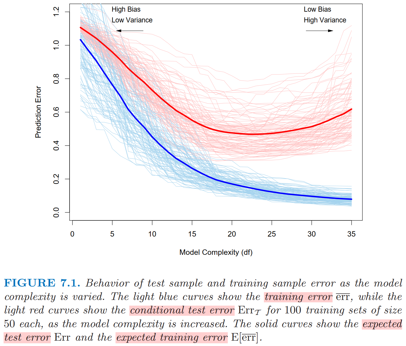
In the Figure, Lasso is used to produce the fits. Model complexity is the number of variables used (in linear settings).
- Training error is not a good estimate of the test error, as seen in Figure above.
There is some intermediate model complexity that gives minimum expected test error. Training error consistently decreases with model complexity, typically dropping to zero if we increase the model complexity enough. However, a model with zero training error is overfit to the training data and will typically generalize poorly.
Conditional or Expected Test Error
Test error \(\operatorname{Err}_{\mathcal{T}}\) in \(\eqref{eq:test_error}\) is the error conditional on a given training set \(\mathcal{T}\), as opposed to the expected test error \(\operatorname{Err}\) in \(\eqref{eq:expected_test_error}\) which is an average over all sorts of training sets (we’re may never going to get to use).
\(\mathrm{Err}\) is more amenable to statistical analysis than the conditional one, and most methods effectively estimate the expected error. It does not seem possible to estimate conditional error effectively, given only the information in the same training set.
Simulation
Model setting: linear model with \(10\) true variables.
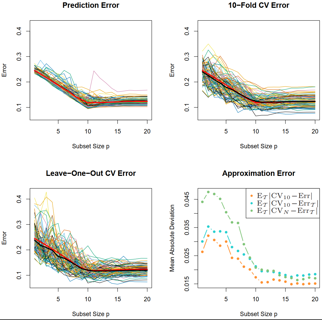
Figure. The thick red curve is the expected prediction error \(\mathrm{Err}\) . While, the thick black curves are the expected CV curves \(\mathrm{E}_{\mathcal{T}}\mathrm{CV}_{10}\) and \(\mathrm{E}_{\mathcal{T}}\mathrm{CV}_{n}\) . The lower-right panel shows the mean absolute deviation of the CV curves from the conditional error, \(\mathrm{E}_{\mathcal{T}}\vert\mathrm{CV}_{K}-\mathrm{Err}_{\mathcal{T}}\vert\) , as well as from the expected error \(\mathrm{E}_{\mathcal{T}}\vert\mathrm{CV}_{K}-\mathrm{Err}\vert\) for \(K={10,n}\).
It shows that both 10-fold CV and LOO CV are approximately unbiased for \(\operatorname{Err}\). 10-fold CV performs better than LOO CV.
We conclude that estimation of test error for a particular training set is not easy in general, given just the data from that same training set. Instead, cross-validation and related methods may provide reasonable estimates of the expected error \(\mathrm{Err}\).
This example tells us that in practice, for a given training set, it is difficult for us to estimate the generalization error.
泛化误差上界
统计学习方法 (李航, 第二版, Section 1.6.2) 给出了二分类问题的泛化误差的上界定理.
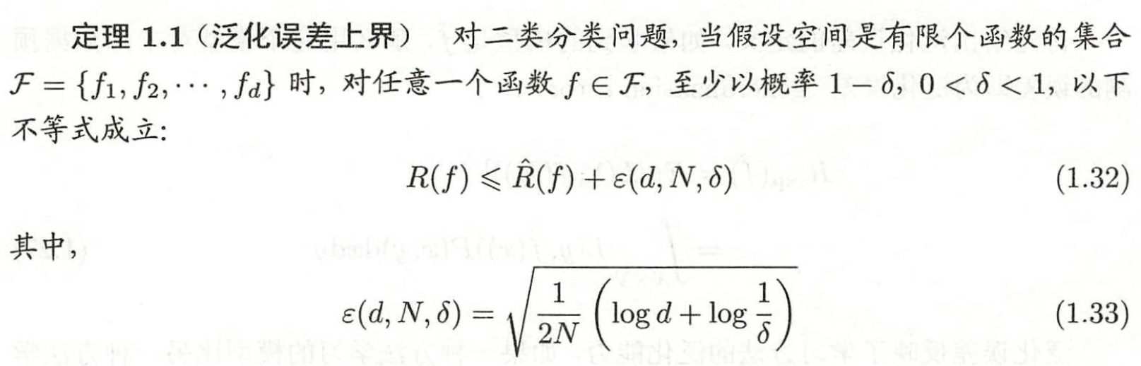
(1.32) 中, 左边是泛化误差, 右边为其上界, 其中 \(\hat{R}(f)\) 为训练误差; \(\varepsilon\) 是一个很小的量, 它随着样本大小 N 递减.
这个定理的条件较严格, 它要求函数空间是有限个函数组成的, 而且训练样本从总体中随机抽样. 李航说, 在一般的条件下, 该定理不容易得到.